Reducing Number of Predictors In Predictive Analytics
- Stepwise Regression
- Any Mechanism Using Automated or Manual Steps
Thought Experiment | Find some lucky pennies
Imagine that you have 50 pennies labeled 1 through 50 and you flip each one 10 times and write on each coin how many times it landed head side up.
Set It Up
I should have said, that we are looking for some lucky pennies, because I going to use the lucky pennies we find in a magic trick later. To find a lucky penny, I need to decide how many heads I need to observe to be surprised.
I am going to cheat, because I happen to remember just enough theoretical statistics to know that when you observe a group of boolean trials, you can use the binomial distribution to calculated the probability of observing any number of one type of observation (heads) out of a known number of trials. (We are not going to show the equation, but it’s a combinatorial expression with factorials so it is pretty.)
For the sake of brevity, I am going to tell you it takes a lot to surprise me.
This Is Surprising Enough (I think ??)
I am going to be a traditionalist here and decide I will be surprised if there are 8 or more heads out of 10 tosses.
What Did We Just Accomplish?
- I am pleased that I found so many valuable pennies out of 50.
- I have thoughtfully recorded how many heads I observed on each lucky penny so I do not need to do all that sampling stuff again.
I can confidently carry these pennies into my magic show knowing they will continue to perform as well there as they did here.
But We are Statisticians
## [1] 2.049443e-86## [1] 0.0006958708## [1] 0.05337477## [1] 0.04684365Now as statisticians, 10 is not a big enough sample for a good estimate so let’s make it bigger.
We’re Still Surprised
surprise_threshhold_large <- 526
results_large <- rbinom(n_coins, tosses_large, p_heads)
picks_large <- seq_along(results_large)[results_large >= surprise_threshhold_large]
length(picks_large)
## [1] 4## [1] 5 15 26 39## [1] 528 533 531 539What Have We Seen?
- Root cause of where stepwise methods go wrong
It is not the initial sample, the results of flipping the 50 coins. It is the belief that the coins that behaved in a surprising way will continue to behave in a surprising way.
Stepwise Methods
- Forward Selection
- Sequentially adds predictors having the most effect
- Stop when no significant improvement can be obtained
Stepwise Methods
- Backward Selection
- Starts with full model
- Predictors are removed one by one based on the least effect (\(F\) statistic)
- Stop when all remaining predictors have F statistics at least as large as a stay threshold
Stepwise Methods
- Stepwise Selection
- Sequentially adds predictors having the most effect and greater than entry threshold
- Removes predictors with effect less than stay threshold
- Optional: Stop when no significant improvement can be obtained
Statistical Issues
- Yields \(R^2\) values that are biased to be high
- Based on methods (e.g., \(F\) tests for nested models) intended to be used to test prespecified hypotheses
- \(F\) and \(\chi^2\) tests do not have their claimed distributions
- Yields \(p\)-values that do not have the proper meaning
- Gives biased regression coefficients that need shrinkage
Effects Demonstrated in 1970’s and 1980’s
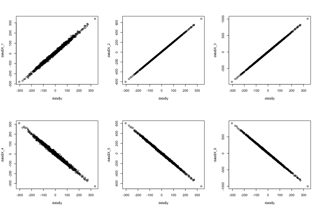
- Has severe problems in the presence of collinearity
- Does not select model having minumum mean residual squared error
- Users often attribute relative importance to order of when variables go in and out of model
Effects Demonstrated in 1992 (1 of 6)
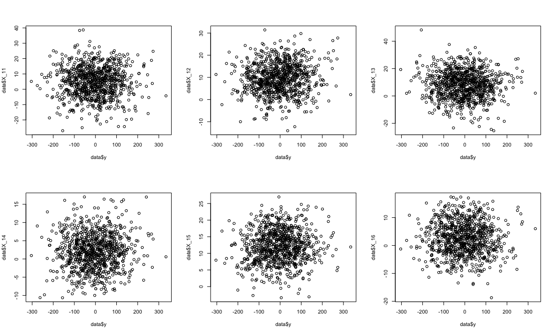
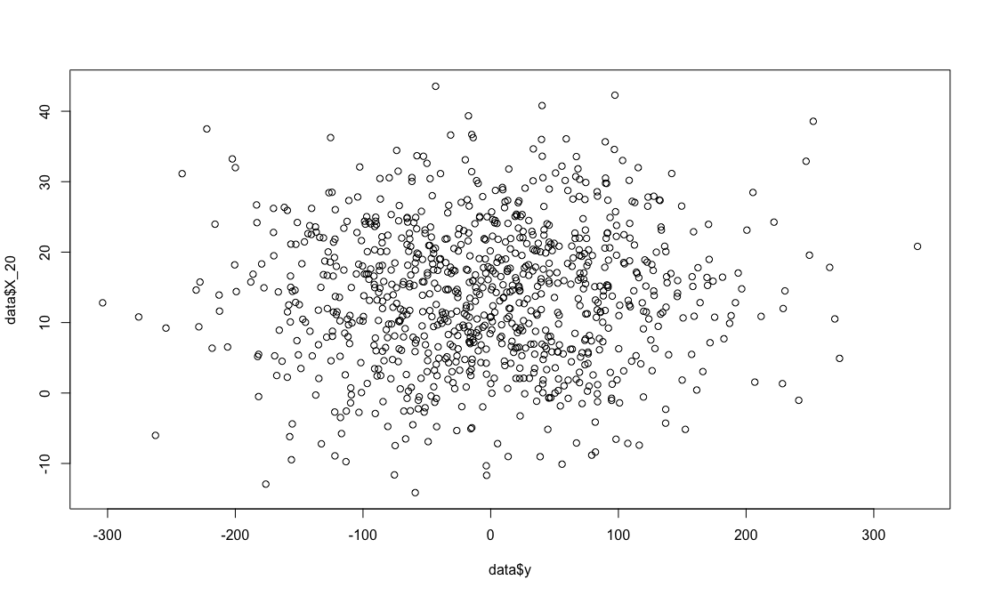
- Number of candidate predictor variables affected the number of noise variables that gained entry to the model
Effects Demonstrated in 1992 (2 of 6)
-
Number of candidate predictor variables affected the number of noise variables that gained entry to the model
Predictors Noise %Noise 12 0.43 20 18 0.96 40 24 1.44 46
Effects Demonstrated in 1992 (3 of 6)
-
Number of candidate predictor variables affected the number of noise variables that gained entry to the model
- Effect of multicollinearity (correlation of 0.4)
Predictors Noise %Noise 12 0.47 35 18 0.93 59 24 1.36 62
Effects Demonstrated in 1992 (4 of 6)
-
Number of candidate predictor variables affected the number of noise variables that gained entry to the model
Predictors Actual Noise %Noise 12 1.70 0.43 20 18 1.64 0.96 40 24 1.66 1.44 46
Effects Demonstrated in 1992 (5 of 6)
-
Number of candidate predictor variables affected the number of noise variables that gained entry to the model
- Effect of multicollinearity (correlation of 0.4)
Predictors Actual Noise %Noise 12 0.86 0.47 35 18 0.87 0.93 59 24 0.83 1.36 62
Effects Demonstrated in 1992 (6 of 6)
- Number of candidate predictor variables affected the number of noise variables that gained entry to the model
- Authentic variables selected less than \(0.5\) the time
- Noise variables selected \(0.20\) to \(0.74\) of the time
- Increasing sample size does not help much
- \(R^2 \propto\) number candidate predictor variables and not the number of final predictor variables
- Method yields confidence intervals for effects and predicted values that are falsely narrow
What If You Change Thresholds
\(N = 900\)
| Predictors | Noise \(\alpha = 0.0016\) | Noise \(\alpha = 0.15\) |
|---|---|---|
| 12 | 2 | 2 |
| 18 | 3 | 3 |
| 24 | 4 | 4 |
| 50 | 8 | 10 |
| 100 | 16 | 17 |