Comprehensive Tutorial: Stochastic Reserving Models

R. Mark Sharp

2026-01-24

Introduction

This tutorial demonstrates all five stochastic reserving models implemented in the stochasticreserver package: 1. Chain Ladder - Standard development factor approach 2. Cape Cod (Bornhuetter-Ferguson variant) - Exposure-based method 3. Berquist-Sherman - Incremental severity method with trend 4. Hoerl Curve - Smooth curve with shared operational time parameters 5. Wright - Generalized Hoerl with individual accident year levels

These methods are based on Roger Hayne’s paper “A Flexible Framework for Stochastic Reserving Models” published in Variance journal (PDF). The key insight is that all five methods can be unified under a common maximum likelihood estimation framework, enabling consistent uncertainty quantification.

Theoretical Framework

Uncertainty in Loss Reserving

Loss reserve estimates face three distinct sources of uncertainty:

1. Process Uncertainty - Inherent stochastic fluctuation in outcomes even when parameters are known exactly. This represents the irreducible randomness in insurance claim development.

2. Parameter Uncertainty - Error from estimating unknown parameters. Even with the correct model structure, finite data leads to estimation error.

3. Model Uncertainty - Risk that the assumed model structure doesn’t match actual data-generating processes. Different reserving methods may yield different estimates, revealing where assumptions require investigation.

This package addresses process and parameter uncertainty through maximum likelihood estimation (MLE). Model uncertainty is addressed by enabling comparison across multiple methods.

Maximum Likelihood Estimation

MLEs have desirable asymptotic properties (as sample size increases):

• Consistency: Estimates converge to true parameter values
• Efficiency: Variance achieves the theoretical lower bound (Cramér-Rao)
• Asymptotic Normality: Distribution approaches Gaussian with mean $\theta$ and covariance equal to the inverse Fisher information matrix

The Fisher Information Matrix is:

$$I(\theta)_{ij} = E\left[\frac{\partial^2}{\partial\theta_i\partial\theta_j} (-\ln L(X|\theta))\right]$$

This enables uncertainty quantification through the variance-covariance matrix $\Sigma = I(\theta)^{-1}$.

Stochastic Model for Incremental Averages

All models share a common likelihood structure. For incremental averages $A_{ij}$ (where $i$ = accident year, $j$ = development lag), we assume:

$$A_{ij} \sim N(g_{ij}(\theta), \sigma^2_{ij})$$

The expected value $g_{ij}(\theta)$ is model-specific (Chain Ladder, Cape Cod, etc.), while the variance structure is shared:

$$\sigma^2_{ij} = e^{\kappa - w_i} \cdot (g_{ij}(\theta)^2)^p$$

where:

• $\kappa$ is a proportionality constant
• $w_i = \log(d_i)$ where $d_i$ is the exposure count for accident year $i$
• $p$ is a power parameter controlling heteroscedasticity

Negative Log-Likelihood Function

For a single observation, the negative log-likelihood is:

$$\ell(x; \mu, \kappa, p) = \frac{1}{2}\left(\kappa - w + \ln(2\pi(\mu^2)^p)\right) + \frac{(x-\mu)^2}{2e^{\kappa-w}(\mu^2)^p}$$

The total objective function sums over all available cells in the triangle.

The Five Model Forms

Each model specifies a different expected value function $g_{ij}(\theta)$: | Model | Expected Value Form | Parameters | |——-|———————|————| | Chain Ladder | $\theta_j \cdot U_i$ | Development proportions (sum to 1) | | Cape Cod | $\theta_0 \cdot \theta_i^{row} \cdot \theta_j^{col}$ | Level + row/column factors | | Berquist-Sherman | $\theta_i \cdot e^{\theta_{trend} \cdot j}$ | Year levels + trend | | Hoerl Curve | $e^{\alpha + \beta_1\tau + \beta_2\tau^2 + \beta_3\ln(\tau) + \beta_4 i}$ | Curve params + row trend | | Wright | $e^{\alpha_i + \beta_1\tau + \beta_2\tau^2 + \beta_3\ln(\tau)}$ | Individual levels + curve |

where $\tau$ represents operational time (development lag) and $U_i$ represents the ultimate for accident year $i$.

Gradient and Hessian

Efficient optimization requires analytical gradients and Hessians. For parameter vector $\mathbf{a} = (\theta_1, \ldots, \theta_k, \kappa, p)$:

Gradient with respect to model parameters: $$\frac{\partial \ell}{\partial \theta} = \sum_{i,j} g'_{ij}(\theta) \cdot \left(\frac{p}{\mu_{ij}} + \frac{\mu_{ij} - A_{ij}}{\sigma^2_{ij}} - \frac{p(A_{ij} - \mu_{ij})^2}{\sigma^2_{ij} \mu_{ij}}\right)$$

Gradient with respect to variance parameters: $$\frac{\partial \ell}{\partial \kappa} = \frac{1}{2}\sum_{i,j} \left(1 - \frac{(A_{ij} - \mu_{ij})^2}{\sigma^2_{ij}}\right)$$

The Hessian matrix enables Newton-type optimization and provides the information matrix for uncertainty quantification.

library(stochasticreserver)
library(mvtnorm)
library(abind)
library(stats)

Data

Package Data: Hayne’s Example Triangle

The package includes data from the reference paper - a 10x10 development triangle of cumulative averages (B0) and exposure counts (dnom).

# Load the cumulative average triangle
B0 <- stochasticreserver::B0
dnom <- stochasticreserver::dnom
size <- nrow(B0)

# Display the triangle
cat("Cumulative Average Triangle (B0):\n")

## Cumulative Average Triangle (B0):

print(round(B0, 2))

##         [,1]    [,2]    [,3]    [,4]    [,5]    [,6]    [,7]    [,8]    [,9]
##  [1,] 670.26 1480.25 1938.54 2466.25 2837.85 3003.52 3055.39 3132.94 3141.19
##  [2,] 767.99 1592.50 2463.79 3019.72 3374.73 3553.61 3602.28 3627.28 3645.57
##  [3,] 740.58 1615.80 2345.85 2910.53 3201.52 3417.71 3506.59 3529.00      NA
##  [4,] 862.12 1754.90 2534.78 3270.85 3739.89 4003.00 4125.31      NA      NA
##  [5,] 840.94 1859.03 2804.55 3445.35 3950.47 4185.95      NA      NA      NA
##  [6,] 848.00 2052.92 3076.14 3861.03 4351.58      NA      NA      NA      NA
##  [7,] 901.77 1927.89 3003.59 3881.42      NA      NA      NA      NA      NA
##  [8,] 935.20 2103.98 3181.75      NA      NA      NA      NA      NA      NA
##  [9,] 759.32 1584.91      NA      NA      NA      NA      NA      NA      NA
## [10,] 723.30      NA      NA      NA      NA      NA      NA      NA      NA
##         [,10]
##  [1,] 3159.73
##  [2,]      NA
##  [3,]      NA
##  [4,]      NA
##  [5,]      NA
##  [6,]      NA
##  [7,]      NA
##  [8,]      NA
##  [9,]      NA
## [10,]      NA

cat("\nExposure Counts (dnom):\n")

## 
## Exposure Counts (dnom):

print(round(dnom, 0))

##  [1] 39161 38672 41801 42263 41481 40214 43599 42118 43479 49492

Data Preparation

We need to prepare several derived quantities for the models:

# Calculate incremental average matrix (A0)
A0 <- cbind(B0[, 1], B0[, 2:size] - B0[, 1:(size - 1)])

# Generate log exposure matrix for variance structure
logd <- log(matrix(dnom, size, size))

# Create row and column index matrices
rowNum <- row(A0)
colNum <- col(A0)

# Create masks for data availability
# upper_triangle_mask: TRUE for cells with available data
upper_triangle_mask <- (size - rowNum) >= colNum - 1

# msn: mask for next forecast diagonal (one-period ahead)
msn <- (size - rowNum) == colNum - 2

# msd: mask for current diagonal (paid to date)
msd <- (size - rowNum) == colNum - 1

# Calculate amount paid to date for each accident year
paid_to_date <- rowSums(B0 * msd, na.rm = TRUE)

cat("Paid to Date by Accident Year:\n")

## Paid to Date by Accident Year:

print(round(paid_to_date, 2))

##  [1] 3159.73 3645.57 3529.00 4125.31 4185.95 4351.58 3881.42 3181.75 1584.91
## [10]  723.30

Simulated Data: Auto Liability Example

To demonstrate the models on different data characteristics, we also create a simulated dataset representing a stylized auto liability triangle. This simulated data exhibits: - Moderate development over 10 periods - Slight trend in accident year severity - Realistic exposure variation

Note: This data is simulated. For production use, replace with actual public data such as triangles from regulatory filings or industry studies.

set.seed(42)

# Simulate a second triangle with different characteristics
simulate_triangle <- function(n_years = 10, base_ult = 5000, trend = 0.03,
                              dev_pattern = NULL) {
  if (is.null(dev_pattern)) {
    # Typical auto liability development pattern
    dev_pattern <- c(0.35, 0.25, 0.15, 0.10, 0.06, 0.04, 0.025, 0.015,
                     0.008, 0.002)
    dev_pattern <- dev_pattern / sum(dev_pattern)  # Normalize
  }

  n_dev <- length(dev_pattern)

  # Generate ultimates with trend
  ultimates <- base_ult * (1 + trend)^(0:(n_years - 1))
  ultimates <- ultimates * exp(rnorm(n_years, 0, 0.05))  # Add noise

  # Generate incremental averages
  incr_avg <- matrix(NA, n_years, n_dev)
  for (i in 1:n_years) {
    for (j in 1:n_dev) {
      if ((n_years - i) >= (j - 1)) {
        mu <- ultimates[i] * dev_pattern[j]
        sigma <- mu * 0.1  # 10% coefficient of variation
        incr_avg[i, j] <- rnorm(1, mu, sigma)
      }
    }
  }

  # Convert to cumulative
  cum_avg <- t(apply(incr_avg, 1, cumsum))

  # Generate exposures (claim counts)
  exposures <- round(runif(n_years, 35000, 50000))

  list(
    B0 = cum_avg,
    A0 = incr_avg,
    dnom = exposures,
    ultimates = ultimates
  )
}

sim_data <- simulate_triangle()
B0_sim <- sim_data$B0
A0_sim <- sim_data$A0
dnom_sim <- sim_data$dnom

cat("Simulated Cumulative Triangle:\n")

## Simulated Cumulative Triangle:

print(round(B0_sim, 2))

##          [,1]    [,2]    [,3]    [,4]    [,5]    [,6]    [,7]    [,8]    [,9]
##  [1,] 2118.72 3763.52 4455.18 4975.73 5292.73 5520.54 5650.60 5709.59 5741.97
##  [2,] 1698.59 2727.28 3465.37 4026.84 4384.17 4575.81 4697.76 4759.62 4801.51
##  [3,] 1769.59 3181.52 4048.89 4644.97 4949.33 5176.31 5288.17 5362.84      NA
##  [4,] 1805.80 2875.26 3724.21 4299.76 4625.90 4868.57 4999.31      NA      NA
##  [5,] 1734.85 3232.60 4024.08 4681.25 5010.93 5255.69      NA      NA      NA
##  [6,] 2082.96 3411.40 4412.53 5026.17 5375.21      NA      NA      NA      NA
##  [7,] 2315.96 4035.05 5009.57 5460.74      NA      NA      NA      NA      NA
##  [8,] 2203.14 3677.04 4612.09      NA      NA      NA      NA      NA      NA
##  [9,] 2594.93 4591.72      NA      NA      NA      NA      NA      NA      NA
## [10,] 2110.66      NA      NA      NA      NA      NA      NA      NA      NA
##        [,10]
##  [1,] 5754.1
##  [2,]     NA
##  [3,]     NA
##  [4,]     NA
##  [5,]     NA
##  [6,]     NA
##  [7,]     NA
##  [8,]     NA
##  [9,]     NA
## [10,]     NA

Helper Functions

We define helper functions to streamline the analysis across all models.

#' Fit a stochastic reserving model
#'
#' @param model_name Character: "Chain", "CapeCod", "Berquist", "Hoerl",
#'   or "Wright"
#' @param B0 Cumulative average matrix
#' @param A0 Incremental average matrix
#' @param dnom Exposure vector
#' @param paid_to_date Paid amounts to date
#' @param upper_triangle_mask Logical mask for available data
#' @return List with fitted model results
fit_model <- function(model_name, B0, A0, dnom, paid_to_date,
                      upper_triangle_mask) {

  size <- nrow(B0)
  logd <- log(matrix(dnom, size, size))

  # Select model
  model_lst <- switch(model_name,
    "Chain" = chain(B0, paid_to_date, upper_triangle_mask),
    "CapeCod" = capecod(B0, paid_to_date, upper_triangle_mask),
    "Berquist" = berquist(B0, paid_to_date, upper_triangle_mask),
    "Hoerl" = hoerl(B0, paid_to_date, upper_triangle_mask),
    "Wright" = wright(B0, paid_to_date, upper_triangle_mask)
  )

  g_obj <- model_lst$g_obj
  g_grad <- model_lst$g_grad
  g_hess <- model_lst$g_hess
  a0 <- model_lst$a0

  # Get starting values for kappa and p
  E <- g_obj(a0)
  yyy <- (A0 - E)^2
  yyy <- logd + log(((yyy != 0) * yyy) - (yyy == 0))
  sss <- na.omit(data.frame(x = c(log(E^2)), y = c(yyy)))
  if (nrow(sss) > 2) {
    ttt <- array(coef(lm(sss$y ~ sss$x)))[1:2]
  } else {
    ttt <- c(10, 1)
  }
  a0 <- c(a0, ttt)

  # Objective functions
  l.obj <- function(a, A) {
    make_negative_log_likelihood(a, A, dnom, g_obj)
  }

  l.grad <- function(a, A) {
    make_gradient_of_objective(a, A, dnom, g_obj, g_grad)
  }

  l.hess <- function(a, A) {
    make_log_hessian(a, A, dnom, g_obj, g_grad, g_hess)
  }

  # Minimize
  max_ctrl <- list(iter.max = 10000, eval.max = 10000)
  scale_vec <- abs(1 / (2 * ((a0 * (a0 != 0)) + (1 * (a0 == 0)))))

  mle <- tryCatch(
    nlminb(a0, l.obj, gradient = l.grad, hessian = l.hess,
           scale = scale_vec, A = A0, control = max_ctrl),
    error = function(e) {
      # Fallback without hessian
      nlminb(a0, l.obj, gradient = l.grad,
             scale = scale_vec, A = A0, control = max_ctrl)
    }
  )

  # Extract results
  npar <- length(mle$par) - 2
  p <- mle$par[npar + 2]
  mean_fitted <- g_obj(mle$par[1:npar])
  var_fitted <- exp(-outer(logd[, 1], rep(mle$par[npar + 1], size), "-")) *
    (mean_fitted^2)^p
  stres <- (A0 - mean_fitted) / sqrt(var_fitted)

  # Information matrix and variance-covariance
  hess_final <- l.hess(mle$par, A0)
  inf_mat <- tryCatch(
    solve(hess_final),
    error = function(e) NULL
  )

  list(
    model_name = model_name,
    mle = mle,
    npar = npar,
    mean = mean_fitted,
    var = var_fitted,
    stres = stres,
    g_obj = g_obj,
    vcov = inf_mat,
    logd = logd,
    convergence = mle$convergence
  )
}

#' Calculate forecast reserves
#'
#' @param fit Fitted model object
#' @param dnom Exposure vector
#' @param upper_triangle_mask Mask for available data
#' @return Data frame with reserve estimates
calculate_reserves <- function(fit, dnom, upper_triangle_mask) {
  size <- nrow(fit$mean)

  # Forecast for lower triangle (future payments)
  forecast_mask <- !upper_triangle_mask
  forecast_mean <- fit$mean * forecast_mask
  forecast_var <- fit$var * forecast_mask

  # Total reserve by accident year
  reserve_mean <- rowSums(dnom * forecast_mean, na.rm = TRUE)
  reserve_sd <- sqrt(rowSums(dnom^2 * forecast_var, na.rm = TRUE))

  # Aggregate
  total_mean <- sum(reserve_mean)
  total_sd <- sqrt(sum(dnom^2 * forecast_var, na.rm = TRUE))

  data.frame(
    accident_year = c(1:size, "Total"),
    reserve_mean = c(reserve_mean, total_mean),
    reserve_sd = c(reserve_sd, total_sd),
    cv = c(reserve_sd / pmax(reserve_mean, 1), total_sd / total_mean)
  )
}

#' Run Monte Carlo simulation
#'
#' @param fit Fitted model object
#' @param dnom Exposure vector
#' @param upper_triangle_mask Mask for available data
#' @param nsim Number of simulations
#' @return Matrix of simulated reserves
run_simulation <- function(fit, dnom, upper_triangle_mask, nsim = 5000) {
  if (is.null(fit$vcov)) return(NULL)

  size <- nrow(fit$mean)
  npar <- fit$npar

  # Masks for simulation
  smsk <- aperm(array(c(upper_triangle_mask), c(size, size, nsim)),
                c(3, 1, 2))

  # Sample parameters
  spar <- tryCatch(
    rmvnorm(nsim, fit$mle$par, fit$vcov),
    error = function(e) NULL
  )
  if (is.null(spar)) return(NULL)

  # Simulated means
  esim <- fit$g_obj(spar)

  # Simulated variances
  ksim <- exp(aperm(outer(array(spar[, npar + 1], c(nsim, size)),
                          log(dnom), "-"), c(1, 3, 2)))
  psim <- array(spar[, npar + 2], c(nsim, size, size))
  vsim <- ksim * (esim^2)^psim

  # Simulate future averages
  sim_avg <- array(rnorm(nsim * size * size, c(esim), sqrt(c(vsim))),
                   c(nsim, size, size))

  # Calculate reserves
  sdnm <- t(matrix(dnom, size, nsim))
  reserves <- sdnm * rowSums(sim_avg * !smsk, dims = 2)

  cbind(reserves, Total = rowSums(reserves))
}

Model Fitting: All Five Methods

Now we fit all five models to the Hayne example data.

model_names <- c("Chain", "CapeCod", "Berquist", "Hoerl", "Wright")

results <- list()
for (model_name in model_names) {
  cat("Fitting", model_name, "model...\n")
  results[[model_name]] <- fit_model(
    model_name, B0, A0, dnom, paid_to_date, upper_triangle_mask
  )
  cat("  Convergence:", results[[model_name]]$convergence,
      " Parameters:", results[[model_name]]$npar + 2, "\n")
}

## Fitting Chain model...

##   Convergence: 0  Parameters: 11 
## Fitting CapeCod model...

##   Convergence: 0  Parameters: 21 
## Fitting Berquist model...
##   Convergence: 0  Parameters: 13 
## Fitting Hoerl model...
##   Convergence: 0  Parameters: 7 
## Fitting Wright model...
##   Convergence: 0  Parameters: 15

Model 1: Chain Ladder

The Chain Ladder model represents the standard actuarial approach where development factors link successive development periods. In this stochastic formulation, the expected emergence is parameterized such that development proportions sum to 1.

Parameters

chain_fit <- results[["Chain"]]
cat("Chain Ladder Model\n")

## Chain Ladder Model

cat("==================\n")

## ==================

cat("Number of parameters:", chain_fit$npar + 2, "\n")

## Number of parameters: 11

cat("  - Model parameters:", chain_fit$npar, "(development proportions)\n")

##   - Model parameters: 9 (development proportions)

cat("  - Variance parameters: 2 (kappa, p)\n\n")

##   - Variance parameters: 2 (kappa, p)

# Development pattern implied
npar <- chain_fit$npar
theta <- chain_fit$mle$par[1:npar]
dev_pattern <- c(theta, 1 - sum(theta))
cat("Implied development pattern:\n")

## Implied development pattern:

names(dev_pattern) <- paste0("Lag", seq_along(dev_pattern))
print(round(dev_pattern, 4))

##   Lag1   Lag2   Lag3   Lag4   Lag5   Lag6   Lag7   Lag8   Lag9  Lag10 
## 0.1955 0.2307 0.2077 0.1637 0.1043 0.0555 0.0217 0.0132 0.0030 0.0047

cat("\nCumulative:", round(cumsum(dev_pattern), 4), "\n")

## 
## Cumulative: 0.1955 0.4262 0.6339 0.7976 0.9019 0.9574 0.9791 0.9922 0.9953 1

Fitted Values

cat("\nFitted Mean (expected incremental averages):\n")

## 
## Fitted Mean (expected incremental averages):

print(round(chain_fit$mean, 2))

##         [,1]    [,2]    [,3]   [,4]   [,5]   [,6]   [,7]  [,8]  [,9] [,10]
##  [1,] 617.57  729.07  656.33 517.19 329.57 175.45  68.44 41.59  9.51 15.00
##  [2,] 715.93  845.18  760.86 599.57 382.05 203.39  79.34 48.21 11.03 17.39
##  [3,] 695.14  820.64  738.77 582.16 370.96 197.49  77.04 46.81 10.71 16.89
##  [4,] 823.53  972.20  875.21 689.67 439.47 233.96  91.26 55.46 12.69 20.00
##  [5,] 854.54 1008.81  908.16 715.64 456.02 242.77  94.70 57.55 13.16 20.76
##  [6,] 943.04 1113.30 1002.22 789.76 503.25 267.91 104.51 63.51 14.53 22.91
##  [7,] 951.15 1122.87 1010.84 796.55 507.58 270.22 105.41 64.05 14.65 23.11
##  [8,] 981.03 1158.13 1042.59 821.57 523.52 278.70 108.72 66.07 15.11 23.83
##  [9,] 726.85  858.06  772.46 608.70 387.88 206.49  80.55 48.95 11.20 17.66
## [10,] 723.30  853.88  768.69 605.74 385.99 205.48  80.16 48.71 11.14 17.57

Reserve Estimates

chain_reserves <- calculate_reserves(chain_fit, dnom, upper_triangle_mask)
knitr::kable(chain_reserves, digits = 0,
             caption = "Chain Ladder Reserve Estimates")

Chain Ladder Reserve Estimates

accident_year	reserve_mean	reserve_sd	cv
1	0	0	0
2	672557	473869	1
3	1153495	628724	1
4	3725552	1068158	0
5	7722556	1489549	0
6	19036072	2214503	0
7	42945172	3195515	0
8	77393393	4157471	0
9	92779952	4551418	0
10	147356872	5671774	0
Total	392785621	9447957	0

Model 2: Cape Cod (Bornhuetter-Ferguson)

The Cape Cod model incorporates exposure information through a multiplicative structure with row (accident year) and column (development) factors. This allows for prior information about ultimate severity levels.

Parameters

cc_fit <- results[["CapeCod"]]
cat("Cape Cod Model\n")

## Cape Cod Model

cat("==============\n")

## ==============

cat("Number of parameters:", cc_fit$npar + 2, "\n")

## Number of parameters: 21

cat("  - Model parameters:", cc_fit$npar, "\n")

##   - Model parameters: 19

cat("    - 1 level parameter\n")

##     - 1 level parameter

cat("    -", (size - 1), "row factors\n")

##     - 9 row factors

cat("    -", (size - 1), "column factors\n")

##     - 9 column factors

cat("  - Variance parameters: 2\n")

##   - Variance parameters: 2

Reserve Estimates

cc_reserves <- calculate_reserves(cc_fit, dnom, upper_triangle_mask)
knitr::kable(cc_reserves, digits = 0,
             caption = "Cape Cod Reserve Estimates")

Cape Cod Reserve Estimates

accident_year	reserve_mean	reserve_sd	cv
1	0	0	0
2	675487	478362	1
3	1154053	633975	1
4	3705613	1071770	0
5	7709391	1494876	0
6	19040687	2219174	0
7	42938949	3196213	0
8	77307054	4150959	0
9	92581984	4542194	0
10	147002026	5656751	0
Total	392115245	9434799	0

Model 3: Berquist-Sherman

The Berquist-Sherman model is an incremental severity method that explicitly models trend over development periods. This is particularly useful when development patterns are changing over time.

Parameters

berq_fit <- results[["Berquist"]]
cat("Berquist-Sherman Model\n")

## Berquist-Sherman Model

cat("======================\n")

## ======================

cat("Number of parameters:", berq_fit$npar + 2, "\n")

## Number of parameters: 13

cat("  - Model parameters:", berq_fit$npar, "\n")

##   - Model parameters: 11

cat("    -", size, "accident year averages\n")

##     - 10 accident year averages

cat("    - 1 trend parameter\n")

##     - 1 trend parameter

cat("  - Variance parameters: 2\n\n")

##   - Variance parameters: 2

# Extract trend parameter
trend_param <- berq_fit$mle$par[size + 1]
cat("Estimated trend parameter:", round(trend_param, 4), "\n")

## Estimated trend parameter: 0.0452

cat("This implies", round((exp(trend_param) - 1) * 100, 2),
    "% change per development period\n")

## This implies 4.62 % change per development period

Reserve Estimates

berq_reserves <- calculate_reserves(berq_fit, dnom, upper_triangle_mask)
knitr::kable(berq_reserves, digits = 0,
             caption = "Berquist-Sherman Reserve Estimates")

Berquist-Sherman Reserve Estimates

accident_year	reserve_mean	reserve_sd	cv
1	0	0	0
2	643872	337239	1
3	1258406	465360	0
4	3553041	889597	0
5	7338748	1384118	0
6	17011031	2408663	0
7	40234557	4133010	0
8	74139470	6077538	0
9	126323652	8355660	0
10	209606332	11101836	0
Total	480109108	15997662	0

Model 4: Hoerl Curve

The Hoerl model uses a smooth mathematical curve to describe development rather than discrete factors. The curve includes polynomial and logarithmic terms in operational time, plus a row trend.

Mathematical Form

$$\mu_{ij} = \exp(\alpha + \beta_1 \tau_j + \beta_2 \tau_j^2 + \beta_3 \log(\tau_j) + \beta_4 \cdot i)$$

where $\tau_j$ is the development lag (operational time).

Parameters

hoerl_fit <- results[["Hoerl"]]
cat("Hoerl Curve Model\n")

## Hoerl Curve Model

cat("=================\n")

## =================

cat("Number of parameters:", hoerl_fit$npar + 2, "\n")

## Number of parameters: 7

cat("  - Model parameters:", hoerl_fit$npar, "\n")

##   - Model parameters: 5

cat("    - alpha (intercept)\n")

##     - alpha (intercept)

cat("    - beta1 (linear in tau)\n")

##     - beta1 (linear in tau)

cat("    - beta2 (quadratic in tau)\n")

##     - beta2 (quadratic in tau)

cat("    - beta3 (log tau)\n")

##     - beta3 (log tau)

cat("    - beta4 (row trend)\n")

##     - beta4 (row trend)

cat("  - Variance parameters: 2\n\n")

##   - Variance parameters: 2

hoerl_theta <- hoerl_fit$mle$par[1:5]
names(hoerl_theta) <- c("alpha", "beta1", "beta2", "beta3", "beta4")
print(round(hoerl_theta, 4))

##   alpha   beta1   beta2   beta3   beta4 
##  6.4977  0.0034 -0.0652  0.5984  0.0430

Reserve Estimates

hoerl_reserves <- calculate_reserves(hoerl_fit, dnom, upper_triangle_mask)
knitr::kable(hoerl_reserves, digits = 0,
             caption = "Hoerl Curve Reserve Estimates")

Hoerl Curve Reserve Estimates

accident_year	reserve_mean	reserve_sd	cv
1	0	0	0
2	169866	296971	2
3	810147	652176	1
4	2690392	1195122	0
5	7354087	1986075	0
6	17306357	3060366	0
7	40013505	4670729	0
8	72642848	6311653	0
9	124351004	8275308	0
10	207051137	10691966	0
Total	472389343	16115325	0

Model 5: Wright (Generalized Hoerl)

The Wright model extends the Hoerl curve by allowing individual level parameters for each accident year rather than just a linear trend. This provides more flexibility at the cost of additional parameters.

Mathematical Form

$$\mu_{ij} = \exp(\alpha_i + \beta_1 \tau_j + \beta_2 \tau_j^2 + \beta_3 \log(\tau_j))$$

where $\alpha_i$ is an individual intercept for each accident year.

Parameters

wright_fit <- results[["Wright"]]
cat("Wright Model\n")

## Wright Model

cat("============\n")

## ============

cat("Number of parameters:", wright_fit$npar + 2, "\n")

## Number of parameters: 15

cat("  - Model parameters:", wright_fit$npar, "\n")

##   - Model parameters: 13

cat("    -", size, "individual year levels (alpha_i)\n")

##     - 10 individual year levels (alpha_i)

cat("    - 3 operational time parameters (beta1, beta2, beta3)\n")

##     - 3 operational time parameters (beta1, beta2, beta3)

cat("  - Variance parameters: 2\n\n")

##   - Variance parameters: 2

wright_theta <- wright_fit$mle$par[1:wright_fit$npar]
cat("Accident year levels:\n")

## Accident year levels:

print(round(wright_theta[1:size], 4))

##  [1] 6.3169 6.4758 6.4403 6.5919 6.6407 6.7428 6.7468 6.7756 6.4808 6.4732

cat("\nOperational time parameters:\n")

## 
## Operational time parameters:

names(wright_theta[(size + 1):(size + 3)]) <- c("beta1", "beta2", "beta3")
print(round(wright_theta[(size + 1):(size + 3)], 4))

## [1]  0.1864 -0.0776  0.2975

Reserve Estimates

wright_reserves <- calculate_reserves(wright_fit, dnom, upper_triangle_mask)
knitr::kable(wright_reserves, digits = 0,
             caption = "Wright Model Reserve Estimates")

Wright Model Reserve Estimates

accident_year	reserve_mean	reserve_sd	cv
1	0	0	0
2	137270	432966	3
3	646137	800325	1
4	2533412	1306997	1
5	7277123	1888006	0
6	18702982	2609470	0
7	42231067	3524225	0
8	75946730	4334693	0
9	92611271	4768645	0
10	146554330	5807424	0
Total	386640322	10029257	0

Model Comparison

Reserve Estimates Comparison

comparison <- data.frame(
  Accident_Year = 1:size,
  Chain = chain_reserves$reserve_mean[1:size],
  CapeCod = cc_reserves$reserve_mean[1:size],
  Berquist = berq_reserves$reserve_mean[1:size],
  Hoerl = hoerl_reserves$reserve_mean[1:size],
  Wright = wright_reserves$reserve_mean[1:size]
)

# Add totals
comparison <- rbind(
  comparison,
  data.frame(
    Accident_Year = "Total",
    Chain = chain_reserves$reserve_mean[size + 1],
    CapeCod = cc_reserves$reserve_mean[size + 1],
    Berquist = berq_reserves$reserve_mean[size + 1],
    Hoerl = hoerl_reserves$reserve_mean[size + 1],
    Wright = wright_reserves$reserve_mean[size + 1]
  )
)

knitr::kable(comparison, digits = 0,
             caption = "Reserve Comparison Across Models")

Reserve Comparison Across Models

Accident_Year	Chain	CapeCod	Berquist	Hoerl	Wright
1	0	0	0	0	0
2	672557	675487	643872	169866	137270
3	1153495	1154053	1258406	810147	646137
4	3725552	3705613	3553041	2690392	2533412
5	7722556	7709391	7338748	7354087	7277123
6	19036072	19040687	17011031	17306357	18702982
7	42945172	42938949	40234557	40013505	42231067
8	77393393	77307054	74139470	72642848	75946730
9	92779952	92581984	126323652	124351004	92611271
10	147356872	147002026	209606332	207051137	146554330
Total	392785621	392115245	480109108	472389343	386640322

Parameter Count Comparison

param_df <- data.frame(
  Model = model_names,
  Model_Params = sapply(results, function(x) x$npar),
  Variance_Params = 2,
  Total_Params = sapply(results, function(x) x$npar + 2),
  Convergence = sapply(results, function(x) x$convergence)
)
knitr::kable(param_df, caption = "Parameter Count by Model")

Parameter Count by Model

	Model	Model_Params	Variance_Params	Total_Params	Convergence
Chain	Chain	9	2	11	0
CapeCod	CapeCod	19	2	21	0
Berquist	Berquist	11	2	13	0
Hoerl	Hoerl	5	2	7	0
Wright	Wright	13	2	15	0

Negative Log-Likelihood Comparison

nll_df <- data.frame(
  Model = model_names,
  NegLogLik = sapply(results, function(x) x$mle$objective),
  AIC = sapply(results, function(x) {
    2 * (x$npar + 2) + 2 * x$mle$objective
  }),
  BIC = sapply(results, function(x) {
    n_obs <- sum(!is.na(A0) & upper_triangle_mask)
    log(n_obs) * (x$npar + 2) + 2 * x$mle$objective
  })
)
nll_df <- nll_df[order(nll_df$AIC), ]
knitr::kable(nll_df, digits = 2, row.names = FALSE,
             caption = "Model Fit Statistics (sorted by AIC)")

Model Fit Statistics (sorted by AIC)

Model	NegLogLik	AIC	BIC
Chain	288.69	599.37	621.45
Wright	291.16	612.33	642.44
CapeCod	288.66	619.32	661.47
Hoerl	312.86	639.71	653.76
Berquist	308.72	643.45	669.54

Diagnostic Plots

Residual Analysis

Standardized residuals should be approximately standard normal if the model fits well.

par(mfrow = c(3, 2))

for (model_name in model_names) {
  fit <- results[[model_name]]
  stres <- fit$stres

  # Q-Q plot
  qqnorm(c(stres), main = paste(model_name, "- Q-Q Plot"))
  qqline(c(stres), col = "red")
}

# Combined residual comparison
par(mfrow = c(1, 1))

Residuals by Calendar Year

par(mfrow = c(2, 3))

for (model_name in model_names) {
  fit <- results[[model_name]]
  stres <- fit$stres
  cy <- rowNum + colNum - 1

  plot(c(cy), c(stres),
       main = paste(model_name, "- by Calendar Year"),
       xlab = "Calendar Year", ylab = "Std Residual",
       pch = 16, col = "blue")
  abline(h = 0, col = "gray")

  # Add mean by CY
  cy_means <- tapply(c(stres), c(cy), mean, na.rm = TRUE)
  lines(as.numeric(names(cy_means)), cy_means, col = "red", lwd = 2)
}

par(mfrow = c(1, 1))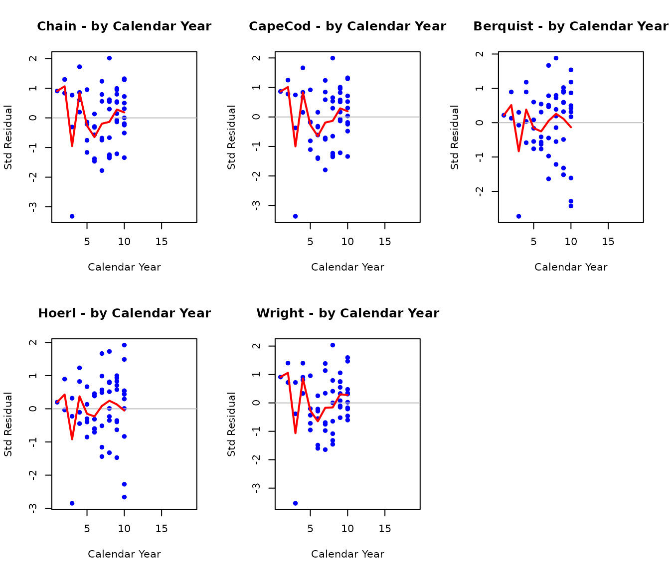

Residuals by Development Lag

par(mfrow = c(2, 3))

for (model_name in model_names) {
  fit <- results[[model_name]]
  stres <- fit$stres

  plot(c(colNum), c(stres),
       main = paste(model_name, "- by Lag"),
       xlab = "Development Lag", ylab = "Std Residual",
       pch = 16, col = "darkgreen")
  abline(h = 0, col = "gray")

  # Add mean by lag
  lag_means <- colMeans(stres, na.rm = TRUE)
  lines(1:size, lag_means, col = "red", lwd = 2)
}

par(mfrow = c(1, 1))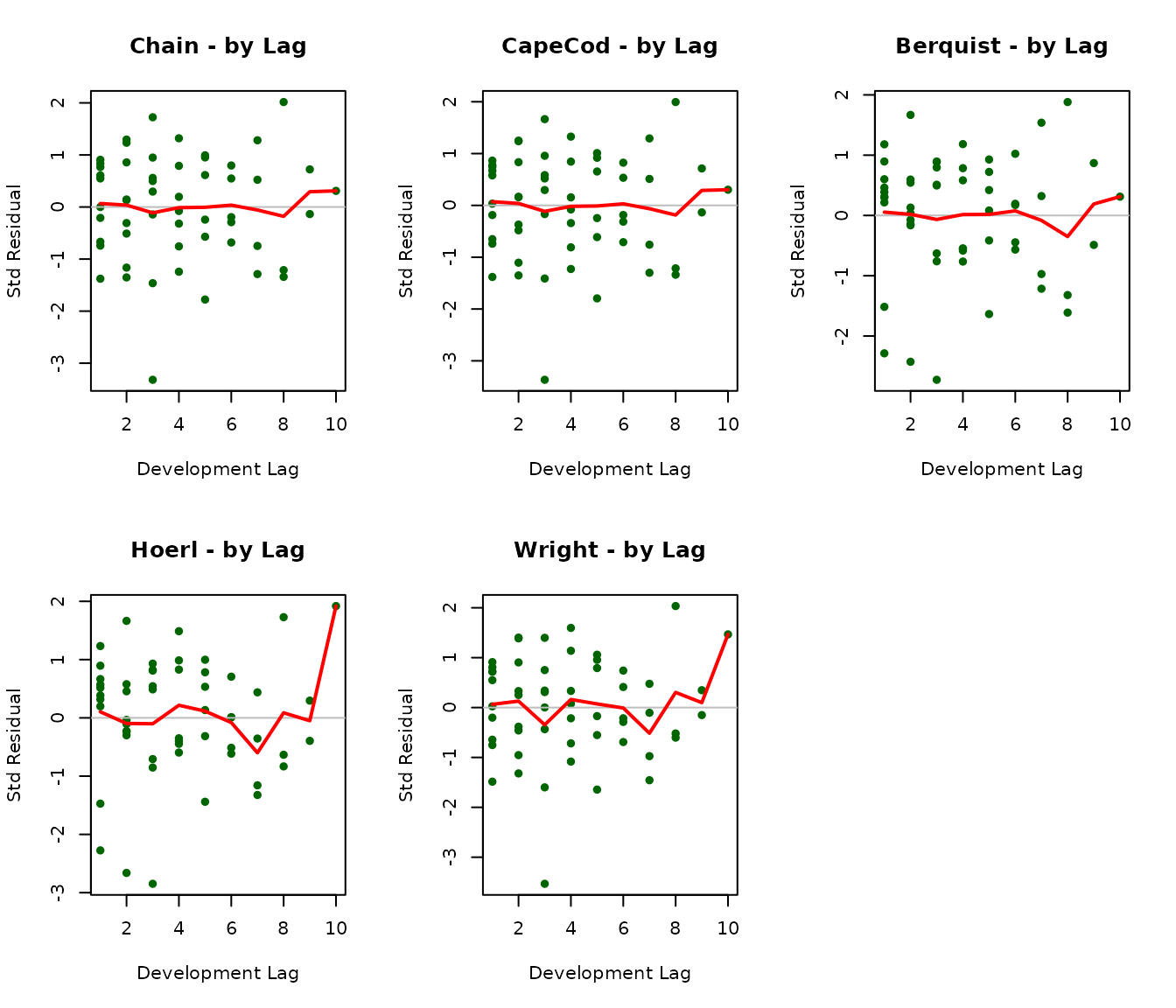

Monte Carlo Simulation

We run simulations to generate full reserve distributions for each model.

set.seed(123)
nsim <- 5000

sim_results <- list()
for (model_name in model_names) {
  cat("Running simulation for", model_name, "...\n")
  sim_results[[model_name]] <- run_simulation(
    results[[model_name]], dnom, upper_triangle_mask, nsim
  )
}

## Running simulation for Chain ...
## Running simulation for CapeCod ...
## Running simulation for Berquist ...
## Running simulation for Hoerl ...
## Running simulation for Wright ...

Distribution of Total Reserves

par(mfrow = c(2, 3))

for (model_name in model_names) {
  sim <- sim_results[[model_name]]
  if (!is.null(sim)) {
    hist(sim[, "Total"], breaks = 50, main = model_name,
         xlab = "Total Reserve", col = "lightblue", border = "white")
    abline(v = mean(sim[, "Total"]), col = "red", lwd = 2)
    abline(v = quantile(sim[, "Total"], c(0.05, 0.95)),
           col = "blue", lwd = 2, lty = 2)
  }
}

par(mfrow = c(1, 1))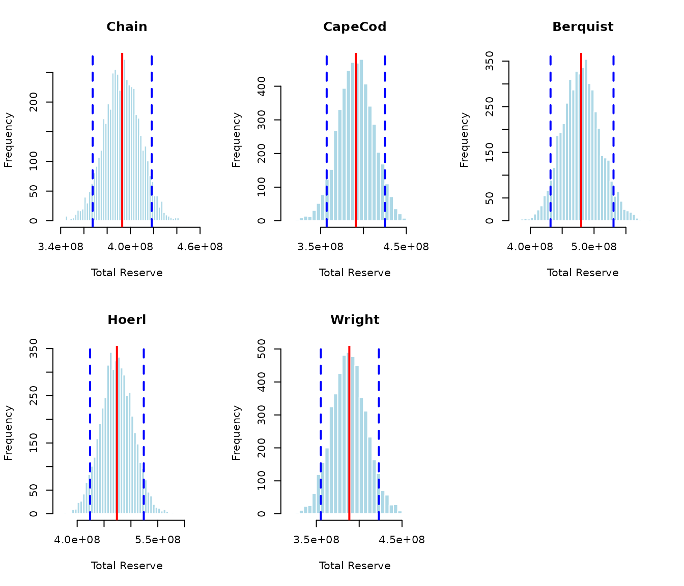

Summary Statistics from Simulation

sim_summary <- data.frame(
  Model = character(),
  Mean = numeric(),
  SD = numeric(),
  CV = numeric(),
  Q05 = numeric(),
  Q50 = numeric(),
  Q95 = numeric(),
  stringsAsFactors = FALSE
)

for (model_name in model_names) {
  sim <- sim_results[[model_name]]
  if (!is.null(sim)) {
    total <- sim[, "Total"]
    sim_summary <- rbind(sim_summary, data.frame(
      Model = model_name,
      Mean = mean(total),
      SD = sd(total),
      CV = sd(total) / mean(total),
      Q05 = quantile(total, 0.05),
      Q50 = quantile(total, 0.50),
      Q95 = quantile(total, 0.95)
    ))
  }
}

knitr::kable(sim_summary, digits = 0, row.names = FALSE,
             caption = "Simulation Summary: Total Reserves")

Simulation Summary: Total Reserves

Model	Mean	SD	CV	Q05	Q50	Q95
Chain	392960259	15561431	0	367489169	393100561	418358515
CapeCod	391119137	20615514	0	357047772	391091786	425096127
Berquist	479838891	29994456	0	431725703	479707042	530528847
Hoerl	473934097	30221127	0	423963049	473631653	523886441
Wright	388494953	20479152	0	355231550	388167747	422943246

Application to Simulated Data

We now apply all models to the simulated auto liability data to demonstrate robustness across different data characteristics.

# Prepare simulated data
size_sim <- nrow(B0_sim)
logd_sim <- log(matrix(dnom_sim, size_sim, size_sim))
rowNum_sim <- row(A0_sim)
colNum_sim <- col(A0_sim)
upper_triangle_mask_sim <- (size_sim - rowNum_sim) >= colNum_sim - 1
msd_sim <- (size_sim - rowNum_sim) == colNum_sim - 1
paid_to_date_sim <- rowSums(B0_sim * msd_sim, na.rm = TRUE)

results_sim <- list()
for (model_name in model_names) {
  cat("Fitting", model_name, "to simulated data...\n")
  results_sim[[model_name]] <- fit_model(
    model_name, B0_sim, A0_sim, dnom_sim, paid_to_date_sim,
    upper_triangle_mask_sim
  )
}

## Fitting Chain to simulated data...

## Fitting CapeCod to simulated data...

## Fitting Berquist to simulated data...
## Fitting Hoerl to simulated data...
## Fitting Wright to simulated data...

Comparison on Simulated Data

comparison_sim <- data.frame(
  Model = model_names,
  Reserve = sapply(results_sim, function(x) {
    res <- calculate_reserves(x, dnom_sim, upper_triangle_mask_sim)
    res$reserve_mean[size_sim + 1]
  }),
  True_IBNR = sum(sim_data$ultimates * dnom_sim) -
    sum(B0_sim * upper_triangle_mask_sim * dnom_sim, na.rm = TRUE)
)
comparison_sim$Error_Pct <- (comparison_sim$Reserve -
  comparison_sim$True_IBNR) / comparison_sim$True_IBNR * 100

knitr::kable(comparison_sim, digits = c(0, 0, 0, 1), row.names = FALSE,
             caption = "Reserve Estimates vs True IBNR (Simulated Data)")

Reserve Estimates vs True IBNR (Simulated Data)

Model	Reserve	True_IBNR	Error_Pct
Chain	466237577	-7763805521	-106.0
CapeCod	458610010	-7763805521	-105.9
Berquist	456073545	-7763805521	-105.9
Hoerl	458513352	-7763805521	-105.9
Wright	464082728	-7763805521	-106.0

Model Selection Guidance

Based on the analysis above, here is guidance for model selection:

When to Use Each Model

1. Chain Ladder: Best for stable, mature lines with consistent development. Fewest parameters (9) provides robustness but less flexibility.

2. Cape Cod: Preferred when you have reliable prior information about ultimate severity levels. The separate row and column factors (19 parameters) provide flexibility but require more data to estimate reliably.

3. Berquist-Sherman: Use when you suspect systematic changes in development patterns over time. The explicit trend parameter (11 total) helps identify and quantify development year trends.

4. Hoerl Curve: Good for smooth development patterns. With only 5 model parameters, it’s parsimonious while still capturing key features. The mathematical form ensures sensible extrapolation.

5. Wright: Most flexible individual year treatment (13 parameters). Use when accident years have genuinely different characteristics that shouldn’t be constrained to a linear trend.

Model Uncertainty

As Hayne emphasizes, practitioners should “use multiple methods” because divergent forecasts indicate where underlying assumptions require investigation. The differences between models reflect model uncertainty - a key component of total reserve uncertainty often underappreciated in practice.

Conclusion

This tutorial demonstrated all five stochastic reserving models in the stochasticreserver package:

• Chain Ladder: Simplest, most constrained
• Cape Cod: Exposure-based with separate factors
• Berquist-Sherman: Explicit development trend
• Hoerl: Smooth parametric curve
• Wright: Individual year levels

The unified maximum likelihood framework enables: 1. Consistent parameter estimation across models 2. Proper uncertainty quantification 3. Model comparison via information criteria 4. Monte Carlo simulation for reserve distributions

For production use, consider: - Running multiple models and comparing results - Examining residual diagnostics carefully - Using simulation to capture parameter uncertainty - Recognizing that model differences indicate structural uncertainty

References

Hayne, R. “A Flexible Framework for Stochastic Reserving Models.” Variance, Vol 7, Issue 2. Available at: https://variancejournal.org/article/120823

Session Information

sessionInfo()

## R version 4.5.2 (2025-10-31)
## Platform: x86_64-pc-linux-gnu
## Running under: Ubuntu 24.04.3 LTS
## 
## Matrix products: default
## BLAS:   /usr/lib/x86_64-linux-gnu/openblas-pthread/libblas.so.3 
## LAPACK: /usr/lib/x86_64-linux-gnu/openblas-pthread/libopenblasp-r0.3.26.so;  LAPACK version 3.12.0
## 
## locale:
##  [1] LC_CTYPE=C.UTF-8       LC_NUMERIC=C           LC_TIME=C.UTF-8       
##  [4] LC_COLLATE=C.UTF-8     LC_MONETARY=C.UTF-8    LC_MESSAGES=C.UTF-8   
##  [7] LC_PAPER=C.UTF-8       LC_NAME=C              LC_ADDRESS=C          
## [10] LC_TELEPHONE=C         LC_MEASUREMENT=C.UTF-8 LC_IDENTIFICATION=C   
## 
## time zone: UTC
## tzcode source: system (glibc)
## 
## attached base packages:
## [1] stats     graphics  grDevices utils     datasets  methods   base     
## 
## other attached packages:
## [1] abind_1.4-8              mvtnorm_1.3-3            stochasticreserver_0.1.1
## 
## loaded via a namespace (and not attached):
##  [1] digest_0.6.39     desc_1.4.3        R6_2.6.1          fastmap_1.2.0    
##  [5] xfun_0.56         cachem_1.1.0      knitr_1.51        htmltools_0.5.9  
##  [9] rmarkdown_2.30    lifecycle_1.0.5   cli_3.6.5         sass_0.4.10      
## [13] pkgdown_2.2.0     textshaping_1.0.4 jquerylib_0.1.4   systemfonts_1.3.1
## [17] compiler_4.5.2    tools_4.5.2       ragg_1.5.0        evaluate_1.0.5   
## [21] bslib_0.9.0       yaml_2.3.12       jsonlite_2.0.0    rlang_1.1.7      
## [25] fs_1.6.6          MASS_7.3-65