Stochastic Reserving with RAA Data
2026-01-22
Introduction
This vignette demonstrates stochastic reserving methods using the RAA (Reinsurance Association of America) claims triangle from the ChainLadder package. This classic dataset contains general liability claims from 1981-1990 with 10 development periods.
The analysis parallels the original stochastic_reserving.Rmd vignette but uses publicly available data instead of the Hayne paper data.
Load Packages and Data
Initialize Triangle
The RAA data is cumulative paid claims in thousands of dollars. Unlike the Hayne paper data, we don’t have exposure counts, so we work directly with total claims rather than averages per exposure.
Show code
# Load RAA cumulative data from package
data(RAA_cumulative)

# Use RAA cumulative data as our development triangle
B0 <- RAA_cumulative

# Since RAA doesn't have exposure data, we use uniform exposure of 1
# This means we're modeling total claims rather than average claims
dnom <- rep(1, nrow(B0))

size <- nrow(B0)

# Display the data
cat("RAA Cumulative Claims Triangle (thousands USD)\n")
RAA Cumulative Claims Triangle (thousands USD)Show code
print(B0) dev
origin 1 2 3 4 5 6 7 8 9 10
1981 5012 8269 10907 11805 13539 16181 18009 18608 18662 18834
1982 106 4285 5396 10666 13782 15599 15496 16169 16704 NA
1983 3410 8992 13873 16141 18735 22214 22863 23466 NA NA
1984 5655 11555 15766 21266 23425 26083 27067 NA NA NA
1985 1092 9565 15836 22169 25955 26180 NA NA NA NA
1986 1513 6445 11702 12935 15852 NA NA NA NA NA
1987 557 4020 10946 12314 NA NA NA NA NA NA
1988 1351 6947 13112 NA NA NA NA NA NA NA
1989 3133 5395 NA NA NA NA NA NA NA NA
1990 2063 NA NA NA NA NA NA NA NA NAModel Selection
Choose which reserving model to use. All five models from the Hayne framework are available:
- Berquist: Berquist-Sherman Incremental Severity
- CapeCod: Cape Cod method
- Hoerl: Generalized Hoerl Curve Model with trend
- Wright: Generalized Hoerl Curve with individual accident year levels
- Chain: Chain Ladder model
Show code
# Select model - try different models by changing this
model <- "Chain"
# model <- "Berquist"
# model <- "CapeCod"
# model <- "Hoerl"
# model <- "Wright"

# Toggle graphs and simulations
graphs <- TRUE
simulation <- TRUE

cat("Selected model:", model, "\n")
Selected model: Chain Show code
cat("Model description:", model_description(model), "\n")Model description: Chain Ladder Model Calculate Incremental Matrix and Masks
Show code
Incremental Claims MatrixShow code
print(A0) 2 3 4 5 6 7 8 9 10
1981 5012 3257 2638 898 1734 2642 1828 599 54 172
1982 106 4179 1111 5270 3116 1817 -103 673 535 NA
1983 3410 5582 4881 2268 2594 3479 649 603 NA NA
1984 5655 5900 4211 5500 2159 2658 984 NA NA NA
1985 1092 8473 6271 6333 3786 225 NA NA NA NA
1986 1513 4932 5257 1233 2917 NA NA NA NA NA
1987 557 3463 6926 1368 NA NA NA NA NA NA
1988 1351 5596 6165 NA NA NA NA NA NA NA
1989 3133 2262 NA NA NA NA NA NA NA NA
1990 2063 NA NA NA NA NA NA NA NA NAShow code
# Generate a matrix to reflect exposure count in the variance structure
logd <- log(matrix(dnom, size, size))

# Set up matrix of rows and columns
rowNum <- row(A0)
colNum <- col(A0)

# Mask matrices
# upper_triangle_mask: allowable data (upper triangular)
# msn: first forecast diagonal
# msd: to-date diagonal
upper_triangle_mask <- (size - rowNum) >= colNum - 1
msn <- (size - rowNum) == colNum - 2
msd <- (size - rowNum) == colNum - 1

# Amount paid to date (cumulative to diagonal)
paid_to_date <- rowSums(B0 * msd, na.rm = TRUE)

cat("\nPaid to date by accident year:\n")
Paid to date by accident year:Show code
print(paid_to_date) 1981 1982 1983 1984 1985 1986 1987 1988 1989 1990
18834 16704 23466 27067 26180 15852 12314 13112 5395 2063 Model-Specific Code
Show code
if (model == "Berquist") {
  model_lst <- berquist(B0, paid_to_date, upper_triangle_mask)
} else if (model == "CapeCod") {
  model_lst <- capecod(B0, paid_to_date, upper_triangle_mask)
} else if (model == "Hoerl") {
  model_lst <- hoerl(B0, paid_to_date, upper_triangle_mask)
} else if (model == "Wright") {
  model_lst <- wright(B0, paid_to_date, upper_triangle_mask)
} else if (model == "Chain") {
  model_lst <- chain(B0, paid_to_date, upper_triangle_mask)
}

g_obj <- model_lst$g_obj
g_grad <- model_lst$g_grad
g_hess <- model_lst$g_hess
a0 <- model_lst$a0
Negative Log-Likelihood Function
The objective function for maximum likelihood estimation. The model has parameters for both the loss model and the variance structure (power parameter and constant of proportionality).
Show code
l.obj <- function(a, A) {
  npar <- length(a) - 2
  e <- g_obj(a[1:npar])
  v <- exp(-outer(logd[, 1], rep(a[npar + 1], size), "-")) * (e^2)^a[npar + 2]
  t1 <- log(2 * pi * v) / 2
  t2 <- (A - e)^2 / (2 * v)
  sum(t1 + t2, na.rm = TRUE)
}

# Gradient of the objective function
l.grad <- function(a, A) {
  npar <- length(a) - 2
  p <- a[npar + 2]
  Av <- aperm(array(A, c(size, size, npar)), c(3, 1, 2))
  e <- g_obj(a[1:npar])
  ev <- aperm(array(e, c(size, size, npar)), c(3, 1, 2))
  v <- exp(-outer(logd[, 1], rep(a[npar + 1], size), "-")) * (e^2)^p
  vv <- aperm(array(v, c(size, size, npar)), c(3, 1, 2))
  dt <- rowSums(g_grad(a[1:npar]) * ((p / ev) + (ev - Av) / vv - p *
                                       (Av - ev)^2 / (vv * ev)),
                na.rm = TRUE,
                dims = 1)
  yy <- 1 - (A - e)^2 / v
  dk <- sum(yy / 2, na.rm = TRUE)
  dp <- sum(yy * log(e^2) / 2, na.rm = TRUE)
  c(dt, dk, dp)
}
Hessian of the Objective Function
-
eis the expected value matrix -
vis the matrix of variances -
A,e,vall have shapec(size, size)
Show code
l.hess <- function(a, A) {
  npar <- length(a) - 2
  p <- a[npar + 2]
  Av <- aperm(array(A, c(size, size, npar)), c(3, 1, 2))
  Am <- aperm(array(A, c(size, size, npar, npar)), c(3, 4, 1, 2))
  e <- g_obj(a[1:npar])
  ev <- aperm(array(e, c(size, size, npar)), c(3, 1, 2))
  em <- aperm(array(e, c(size, size, npar, npar)), c(3, 4, 1, 2))
  v <- exp(-outer(logd[, 1], rep(a[npar + 1], size), "-")) * (e^2)^p
  vv <- aperm(array(v, c(size, size, npar)), c(3, 1, 2))
  vm <- aperm(array(v, c(size, size, npar, npar)), c(3, 4, 1, 2))
  g1 <- g_grad(a[1:npar])
  gg <- aperm(array(g1, c(npar, size, size, npar)), c(4, 1, 2, 3))
  gg <- gg * aperm(gg, c(2, 1, 3, 4))
  gh <- g_hess(a[1:npar])
  dtt <- rowSums(
    gh * (p / em + (em - Am) / vm - p * (Am - em)^2 / (vm * em)) +
      gg * (1 / vm + 4 * p * (Am - em) / (vm * em) +
              p * (2 * p + 1) * (Am - em)^2 / (vm * em^2) - p / em^2),
    dims = 2,
    na.rm = TRUE
  )
  dkt <- rowSums((g1 * (Av - ev) + p * g1 * (Av - ev)^2 / ev) / vv,
                 na.rm = TRUE)
  dtp <- rowSums(g1 * (1 / ev + (log(ev^2) * (Av - ev) +
                                   (p * log(ev^2) - 1) * (Av - ev)^2 / ev) / vv),
                 na.rm = TRUE)
  dkk <- sum((A - e)^2 / (2 * v), na.rm = TRUE)
  dpk <- sum(log(e^2) * (A - e)^2 / (2 * v), na.rm = TRUE)
  dpp <- sum(log(e^2)^2 * (A - e)^2 / (2 * v), na.rm = TRUE)
  m1 <- rbind(array(dkt), c(dtp))
  rbind(cbind(dtt, t(m1)), cbind(m1, rbind(cbind(dkk, c(dpk)), c(dpk, dpp))))
}
Minimization
Starting Values
Use fitted objective function to get starting values for kappa and p parameters.
Actual Minimization
Model Statistics
Show code
Fitted Expected Values (mean): [,1] [,2] [,3] [,4] [,5] [,6] [,7] [,8] [,9] [,10]
[1,] 2458 3914 4010 2975 2087 1791 814 426 273 86
[2,] 2190 3487 3573 2651 1859 1596 726 380 243 77
[3,] 3122 4971 5093 3778 2650 2275 1034 541 346 109
[4,] 3687 5870 6013 4461 3129 2686 1221 639 409 129
[5,] 3734 5945 6091 4519 3170 2721 1237 647 414 131
[6,] 2523 4017 4116 3054 2142 1838 836 437 280 88
[7,] 2266 3608 3697 2743 1924 1651 751 393 251 79
[8,] 3105 4943 5064 3757 2635 2262 1028 538 344 109
[9,] 2081 3314 3395 2519 1767 1516 689 361 231 73
[10,] 2063 3285 3365 2497 1751 1503 683 358 229 72Show code
cat("\nParameter estimates:\n")
Parameter estimates:Variance power (p): 0.6629 Kappa: 3.9023 Information Matrix and Variance-Covariance
Show code
g1 <- g_grad(mle$par[1:npar])
gg <- aperm(array(g1, c(npar, size, size, npar)), c(4, 1, 2, 3))
gg <- gg * aperm(gg, c(2, 1, 3, 4))
meanv <- aperm(array(mean, c(size, size, npar)), c(3, 1, 2))
meanm <- aperm(array(mean, c(size, size, npar, npar)), c(3, 4, 1, 2))
varm <- aperm(array(var, c(size, size, npar, npar)), c(3, 4, 1, 2))

# Masks to screen out NA entries
s <- 0 * A0
sv <- aperm(array(s, c(size, size, npar)), c(3, 1, 2))
sm <- aperm(array(s, c(size, size, npar, npar)), c(3, 4, 1, 2))

# Second derivatives
tt <- rowSums(sm + gg * (1 / varm + 2 * p^2 / (meanm^2)), dims = 2, na.rm = TRUE)
kt <- p * rowSums(sv + g1 / meanv, na.rm = TRUE)
tp <- p * rowSums(sv + g1 * log(meanv^2) / meanv, na.rm = TRUE)
kk <- (1 / 2) * sum(1 + s, na.rm = TRUE)
pk <- (1 / 2) * sum(s + log(mean^2), na.rm = TRUE)
pp <- (1 / 2) * sum(s + log(mean^2)^2, na.rm = TRUE)

# Create information matrix
m1 <- rbind(array(kt), c(tp))
inf <- rbind(cbind(tt, t(m1)), cbind(m1, rbind(c(kk, pk), c(pk, pp))))

# Variance-covariance matrix
vcov <- solve(inf)
Simulation
Run Monte Carlo simulation for distribution of future amounts.
Show code
sim <- matrix(0, 0, 11)
smn <- matrix(0, 0, 11)
spm <- matrix(0, 0, npar + 2)

nsim <- 5000
smsk <- aperm(array(c(upper_triangle_mask), c(size, size, nsim)), c(3, 1, 2))
smsn <- aperm(array(c(msn), c(size, size, nsim)), c(3, 1, 2))

if (simulation) {
  for (i in 1:5) {
    # Randomly generate parameters from multivariate normal
    spar <- rmvnorm(nsim, mle$par, vcov)

    # Arrays to calculate simulated means
    esim <- g_obj(spar)

    # Arrays to calculate simulated variances
    ksim <- exp(aperm(outer(array(spar[, c(npar + 1)], c(nsim, size)),
                            log(dnom), "-"), c(1, 3, 2)))
    psim <- array(spar[, npar + 2], c(nsim, size, size))
    vsim <- ksim * (esim^2)^psim

    # Randomly simulate future values
    temp <- array(rnorm(nsim * size * size, c(esim), sqrt(c(vsim))),
                  c(nsim, size, size))

    # Combine totals by exposure period and aggregate
    sdnm <- t(matrix(dnom, size, nsim))
    fore <- sdnm * rowSums(temp * !smsk, dims = 2)
    forn <- sdnm * rowSums(temp * smsn, dims = 2)

    # Cumulate results
    sim <- rbind(sim, cbind(fore, rowSums(fore)))
    smn <- rbind(smn, cbind(forn, rowSums(forn)))
    spm <- rbind(spm, spar)
  }
}
Results
Reserve Estimates
Show code
cat("Model:", model, "\n")Model: Chain Show code
cat("Description:", model_description(model), "\n\n")Description: Chain Ladder Model Show code
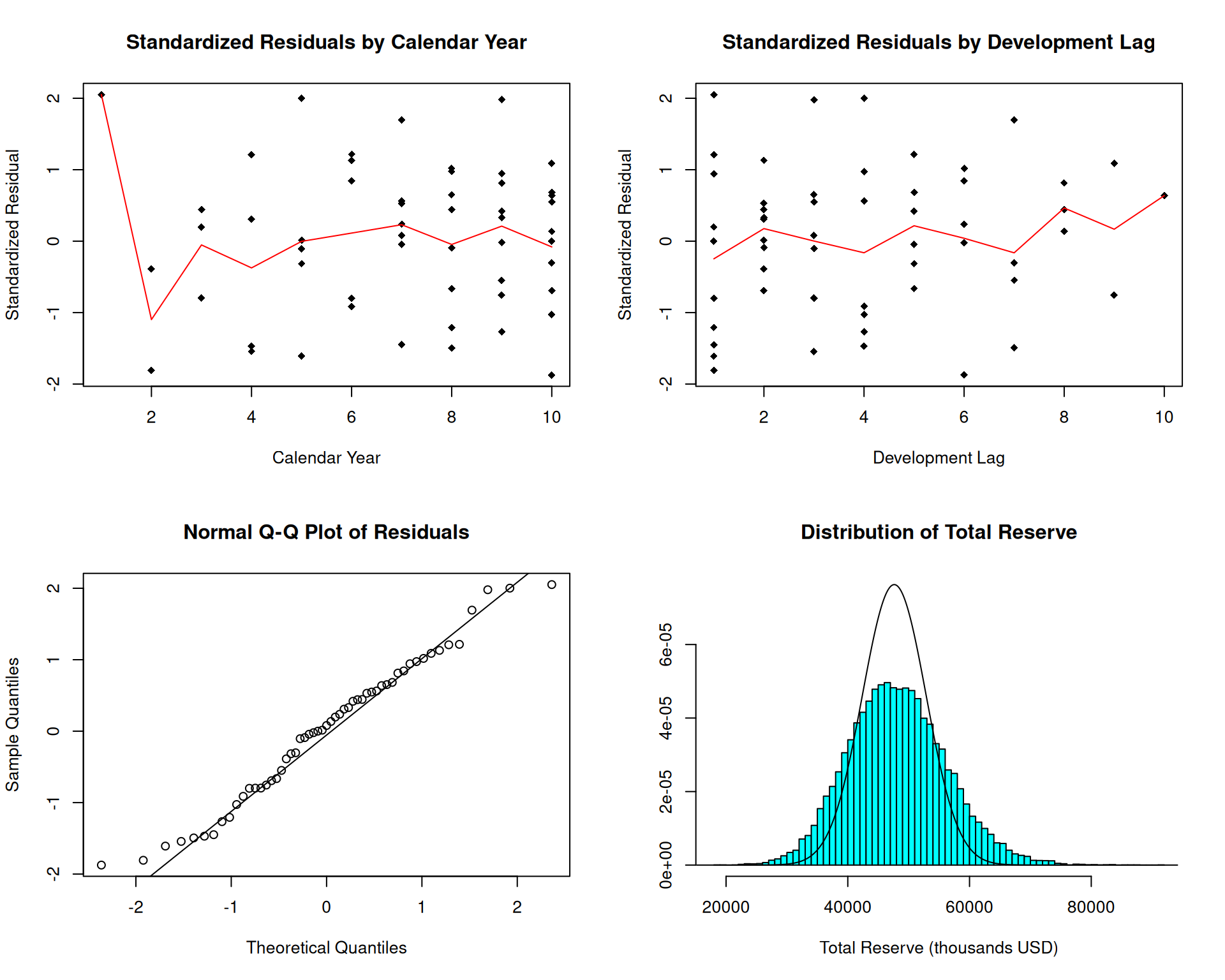
Point Estimate of Total Reserve: 47633 thousand USDShow code
Simulation Summary (Total Reserve):
   Min. 1st Qu.  Median    Mean 3rd Qu.    Max.
  18067   42608   47868   48185   53385   91301
Diagnostic Plots
Show code
if (graphs) {
  # Prep data for lines in scatter plots
  ttt_plot <- array(cbind(c(rowNum + colNum - 1), c(stres)),
                    c(length(c(stres)), 2, 19))
  sss_plot <- t(array(1:19, c(19, length(c(stres)))))

  par(mfrow = c(2, 2))

  # Residuals by Calendar Year
  plot(
    na.omit(cbind(c(rowNum + colNum - 1), c(stres))),
    main = "Standardized Residuals by Calendar Year",
    xlab = "Calendar Year",
    ylab = "Standardized Residual",
    pch = 18
  )
  lines(na.omit(list(
    x = 1:19,
    y = colSums(ttt_plot[, 2, ] * (ttt_plot[, 1, ] == sss_plot), na.rm = TRUE) /
      colSums((ttt_plot[, 1, ] == sss_plot) + 0 * ttt_plot[, 2, ], na.rm = TRUE)
  )), col = "red")

  # Residuals by Lag
  plot(
    na.omit(cbind(c(colNum), c(stres))),
    main = "Standardized Residuals by Development Lag",
    xlab = "Development Lag",
    ylab = "Standardized Residual",
    pch = 18
  )
  lines(na.omit(list(
    x = colNum[1, ],
    y = colSums(stres, na.rm = TRUE) / colSums(1 + 0 * stres, na.rm = TRUE)
  )), col = "red")

  # Q-Q Plot
  qqnorm(c(stres), main = "Normal Q-Q Plot of Residuals")
  qqline(c(stres))

  # Distribution of forecasts
  if (simulation) {
    proc <- list(
      x = (density(sim[, 11]))$x,
      y = dnorm((density(sim[, 11]))$x,
                sum(matrix(c(dnom), size, size) * mean * !upper_triangle_mask),
                sqrt(sum(matrix(c(dnom), size, size)^2 * var * !upper_triangle_mask)))
    )
    MASS::truehist(sim[, 11],
                   ymax = max(proc$y),
                   main = "Distribution of Total Reserve",
                   xlab = "Total Reserve (thousands USD)")
    lines(proc)
  }
}
Simulation Summary by Accident Year
Show code
if (simulation) {
  sumr <- matrix(0, 0, 4)
  sumn <- matrix(0, 0, 4)

  for (i in 1:11) {
    sumr <- rbind(sumr, c(mean(sim[, i]), sd(sim[, i]),
                          quantile(sim[, i], c(.05, .95))))
    sumn <- rbind(sumn, c(mean(smn[, i]), sd(smn[, i]),
                          quantile(smn[, i], c(.05, .95))))
  }

  rownames(sumr) <- c(paste0("AY ", 1981:1990), "Total")
  colnames(sumr) <- c("Mean", "Std Dev", "5%", "95%")

  cat("\nReserve by Accident Year (thousands USD):\n")
  print(round(sumr, 0))

  rownames(sumn) <- c(paste0("AY ", 1981:1990), "Total")
  colnames(sumn) <- c("Mean", "Std Dev", "5%", "95%")

  cat("\nNext Period Forecast by Accident Year (thousands USD):\n")
  print(round(sumn, 0))
}
Reserve by Accident Year (thousands USD):
         Mean Std Dev    5%   95%
AY 1981     0       0     0     0
AY 1982    76     178  -185   374
AY 1983   452     488  -288  1282
AY 1984  1191     850  -148  2630
AY 1985  2434    1276   414  4591
AY 1986  3489    1506  1082  6029
AY 1987  5087    1827  2158  8175
AY 1988 10744    3048  5939 15883
AY 1989 10651    2958  5987 15678
AY 1990 14061    3908  8205 20906
Total   48185    8051 35633 61933

Next Period Forecast by Accident Year (thousands USD):
         Mean Std Dev    5%   95%
AY 1981     0       0     0     0
AY 1982    76     178  -185   374
AY 1983   343     420  -265  1084
AY 1984   649     606  -243  1710
AY 1985  1244     903  -140  2805
AY 1986  1839    1134    57  3800
AY 1987  1939    1156   100  3919
AY 1988  3772    1825   892  6912
AY 1989  3418    1689   739  6275
AY 1990  3365    1715   705  6268
Total   16646    3627 10851 22726
Data Attribution
The RAA data used in this vignette is from the Reinsurance Association of America, obtained via the ChainLadder R package.
Citation: Gesmann M, Murphy D, Zhang Y, Carrato A, Wuthrich M, Concina F, Dal Moro E (2025). ChainLadder: Statistical Methods and Models for Claims Reserving in General Insurance. R package version 0.2.20. https://mages.github.io/ChainLadder/