flowchart LR
  A["Raw studbook<br/>Excel or CSV"] --> B["Quality Control<br/>(Input tab)"]
  B --> C["Pedigree<br/>(Pedigree Browser tab)"]
  C --> D["Potential Parents<br/>tab"]
  C --> E["Age-Sex Pyramid<br/>tab"]
  C --> F["Genetic Value Analysis<br/>tab"]
  C --> G["Breeding Groups<br/>tab"]
  F --> G
  G --> H["Genetic Diversity<br/>tab"]
  F --> H
Purpose, Approach, and a Colony Manager’s Guide to Practice
Source:vignettes/articles/colony-manager-guide.qmd
Abstract
nprcgenekeepr provides genetic tools for primate-colony management: studbook quality control, pedigree construction and browsing, age-sex demographic display, genetic value analysis, and breeding-group formation, delivered through both a Shiny application (runGeneKeepR()) and an exposed R API. This article is a practical, screenshot-illustrated guide for colony managers and primate-center bioinformatics staff, complementing the engineering account in “Engineering nprcgenekeepr 2.0.0” and the seven feature-depth articles listed in Section 4. Section 1 explains why the package exists; Section 2 maps its five function groups onto the app’s tabs and onto the two ways to use them (point-and-click or scripted); Section 3 walks a colony manager through the entire application, tab by tab, using the package’s own shipped example pedigree. This article’s own preparation surfaced and fixed three production issues along the way – an Excel-upload defect that could silently corrupt sire/dam IDs, a “Custom” breeding-group sex ratio option with no numeric input, and a shipped example pedigree missing a column the Potential Parents tab needs to demonstrate populated results – each described where it arose rather than glossed over. All claims in this article are current as of 2026-10-08.
Introduction
This article is an onboarding guide to nprcgenekeepr for the audience it was built for: primate-center bioinformatics staff and colony managers evaluating or learning to use the package. It answers three questions in order – why the package exists, how its capabilities are organized, and what it looks like to actually use it – using the Shiny application (runGeneKeepR()) as the walkthrough’s frame of reference.
It is one of three documents that together cover the package from different angles. “Engineering nprcgenekeepr 2.0.0” documents the modular-architecture migration and development process behind the current application – read it for the how it was built story. Seven shorter feature articles (linked from Section 4’s table) each walk one capability in depth, directly through the R API rather than the Shiny app. This article does neither of those jobs: it is the practical, tab-by-tab guide to using the application as shipped, aimed at a reader who wants to load a pedigree and get results, not read source code.
Scope. Every claim below describing the current application – tab list, control labels, default values, and any number tied to the package’s own data(examplePedigree) example data – was re-verified directly against the source and a live run of the app, as of 2026-09-30. Nothing here is carried forward uncritically from earlier tutorials.
Section 1 – Purpose: Why nprcgenekeepr Exists
The primary goal of nprcgenekeepr is to implement genetic tools for colony management. It was initially conceived and developed as a Shiny web application at the Oregon National Primate Research Center (ONPRC) to facilitate analyses that center routinely performs, and has since been enhanced so that its underlying functions can also be used directly in R scripts rather than only through the Shiny interface (see Section 4’s “two ways to use them”).
Captive breeding colonies – rhesus macaques and other nonhuman primates at National Primate Research Centers – need to manage genetic diversity across generations: avoiding the mating of closely related animals, preserving rare alleles carried by relatively few individuals, and forming breeding groups that balance those genetic goals against real behavioral and housing constraints. nprcgenekeepr’s ranking and grouping methodology follows Vinson and Raboin (2015), A Practical Approach for Designing Breeding Groups to Maximize Genetic Diversity in a Large Colony of Captive Rhesus Macaques (Macaca mulatta), Journal of the American Association for Laboratory Animal Science, 54(6), 700-707.
Work on this package up to and including version 1.0 was supported in part by NIH grants P51 RR13986 to the Southwest National Primate Research Center and P51 OD011092 to the Oregon National Primate Research Center.
Section 2 – Approach: The Five Function Groups and Two Ways to Use Them
nprcgenekeepr’s capability is organized around five function groups. Each maps onto one or more tabs in the Shiny application (walked in Section 5) and, for readers who want to script rather than click, onto a feature article that demonstrates the same underlying functions directly through the R API.
| # | Function group | App tab(s) | Read deeper (R-API walkthrough) |
|---|---|---|---|
| 1 | Quality control of studbooks | Input | Studbook Quality Control |
| 2 | Pedigree construction and browsing, including identifying candidate parents for animals with unknown parentage | Pedigree Browser, Potential Parents | Building a Focal-Animal Pedigree Offline; The Pedigree Diagram Tab |
| 3 | Age-sex demographic display | Age-Sex Pyramid | Age-Sex Pyramid Plots |
| 4 | Genetic value analysis (mean kinship, genome uniqueness) | Genetic Value Analysis, Genetic Value Analysis and Breeding Group Description | Genetic Value Analysis; Validating the Founder-Genome-Equivalent Standard Error |
| 5 | Breeding-group formation and ongoing diversity monitoring | Breeding Groups, Genetic Diversity | Forming Breeding Groups |
The Genetic Diversity and Potential Parents tabs (rows 2 and 5) are recent additions that extend two of the five original groups rather than constituting new ones: Potential Parents extends pedigree construction by proposing candidate parents for animals recorded with unknown parentage; Genetic Diversity extends breeding-group formation by monitoring the diversity of groups once they are formed. Both are covered in Section 5 alongside the tabs they extend.
These five groups compose into one pipeline, from a raw studbook to formed breeding groups:
Two ways to use it. Everything in this pipeline is available both through the Shiny application walked in Section 5 and as directly callable R functions – NAMESPACE exports 233 functions (counted when this article is rendered). An open GitHub issue (#37) tracks, function by function, which exports the Shiny app itself exercises versus which exist primarily for scripted or batch workflows; its own most recent re-verification (2026-06-16) predates the current export count, so treat its exact split as directional rather than a precise current figure. The practical takeaway for this article’s audience: if a task in Section 5 feels like it should be scriptable – batch-processing several pedigrees, or running a workflow without a browser – it very likely already is; the feature articles in Table 1 are worked examples of exactly that.
Section 3 – Practice: A Colony Manager’s Walkthrough
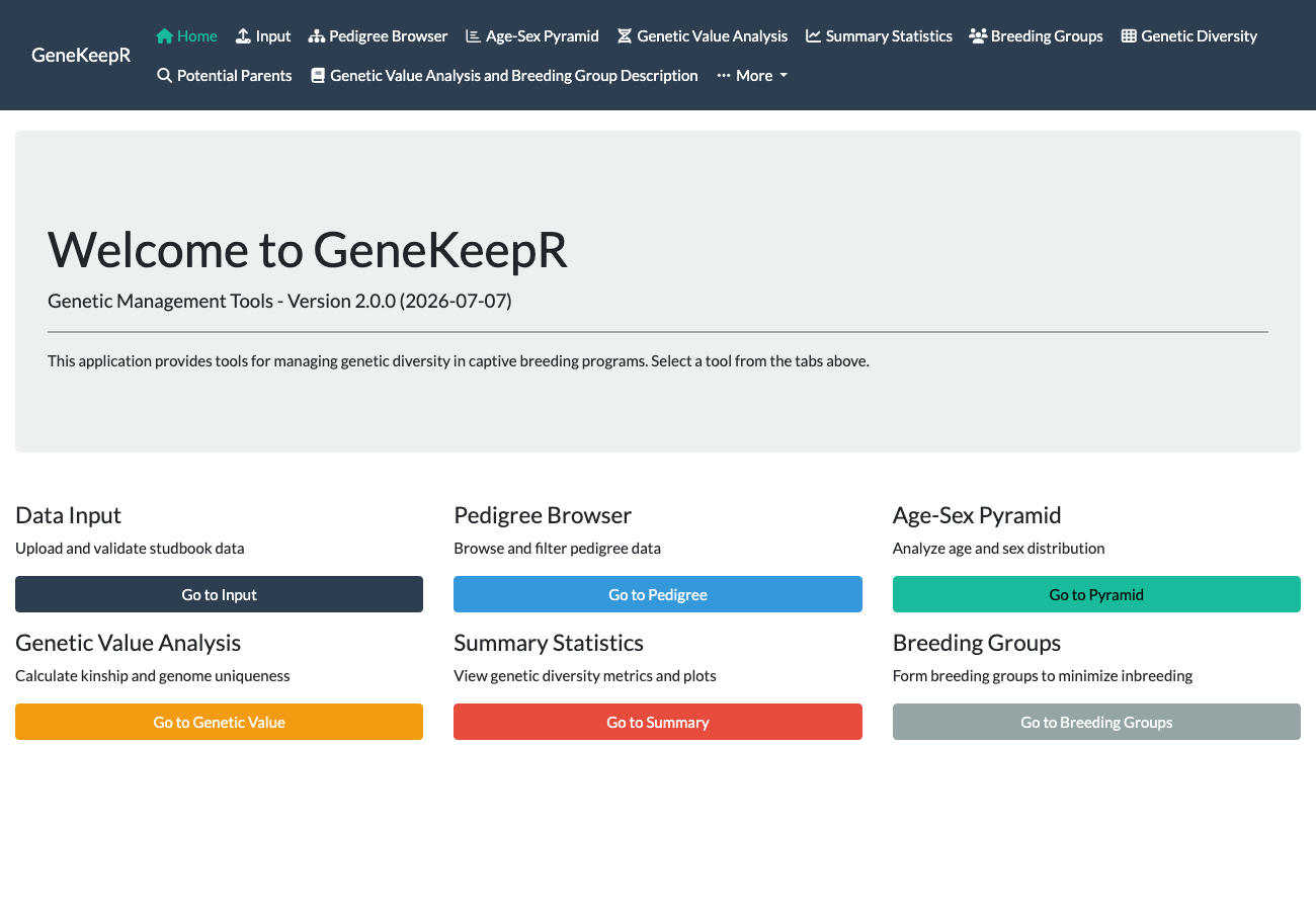
This section walks every tab of the Shiny application in order (except the ONPRC-only ORIP Reporting tab, which appears only on ONPRC installations), using the package’s own shipped example data (data(examplePedigree), data(focalAnimals)) throughout so every step below is reproducible. Start the application with:
(runModularApp() also still launches the application but is deprecated in favor of runGeneKeepR().) The complete online documentation, including the function reference and this article’s companions, is at https://rmsharp.github.io/nprcgenekeepr/.
Uploading a Pedigree File
The Input tab’s “Input Format” sub-tab documents the exact file formats and column requirements accepted – consult it directly rather than a description here, since it is kept in sync with the package’s actual reader code and this article is not.
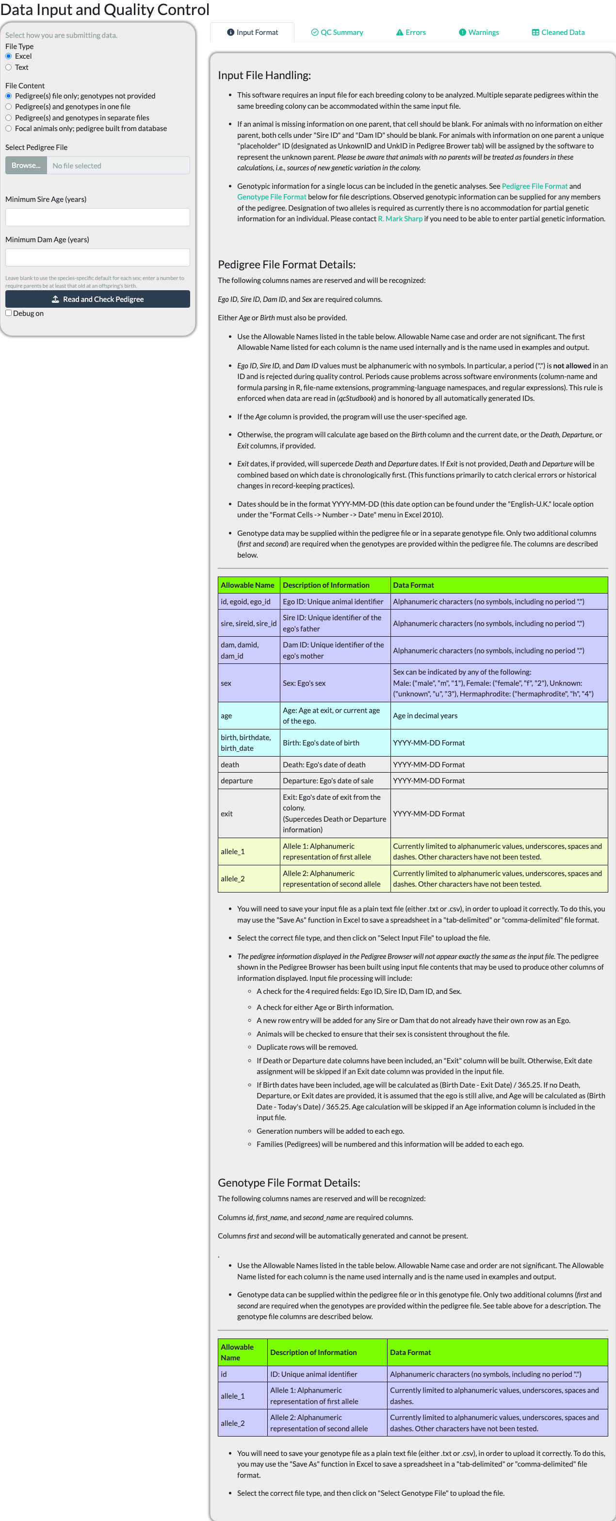
Choose a File Type (Excel or Text) and a File Content option – pedigree only, pedigree and genotypes together or in separate files, or focal animals only (built from a database connection or, offline, from a second uploaded pedigree file) – then browse for the file itself. With “Pedigree(s) and genotypes in one file”, name the two allele columns first and second, first_name and second_name, or allele_1 and allele_2: whole numbers are used as they are and text labels such as A, B, C become whole-number codes, as in a separate genotype file.
Note
Fixed before publication. An earlier draft of this walkthrough found that uploading an Excel workbook shaped like the package’s own shipped example pedigree (several placeholder-parent rows before alphanumeric IDs) silently corrupted the sire/dam columns:
readxlinferred those columns’ type from the early blank rows, guessedlogical, and converted every later alphanumeric ID it could not parse as logical toNA– with no warning surfaced to the user. This affected the same upload path any Excel-format pedigree goes through, not just this example file. Fixed by routing the Excel read through the samecol_types = "text"helper the package’s other Excel readers already use, so both CSV and Excel now round-trip correctly. This walkthrough continues to use CSV below for simplicity, not to work around any remaining defect.
makeExamplePedigreeFile(fileType = "csv")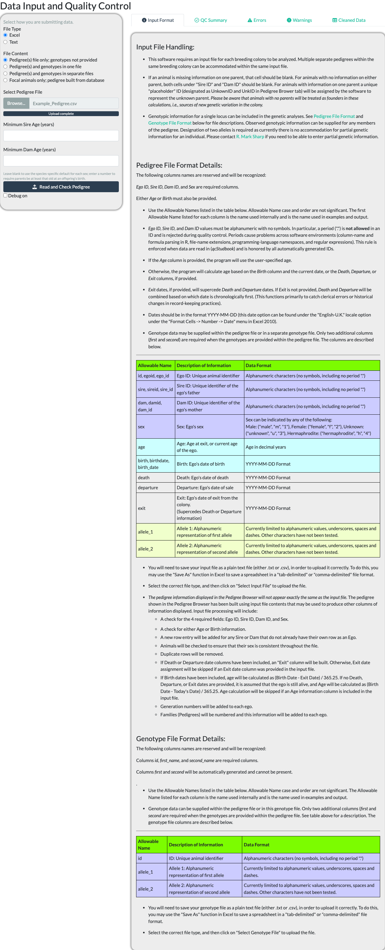
Two optional fields, Minimum Sire Age and Minimum Dam Age, are each left blank by default so that a species- and sex-specific breeding-age default is used automatically; type a number in either field to override that sex’s floor (for macaques, which may reproduce as early as two years of age, a value of 2 is appropriate for both).
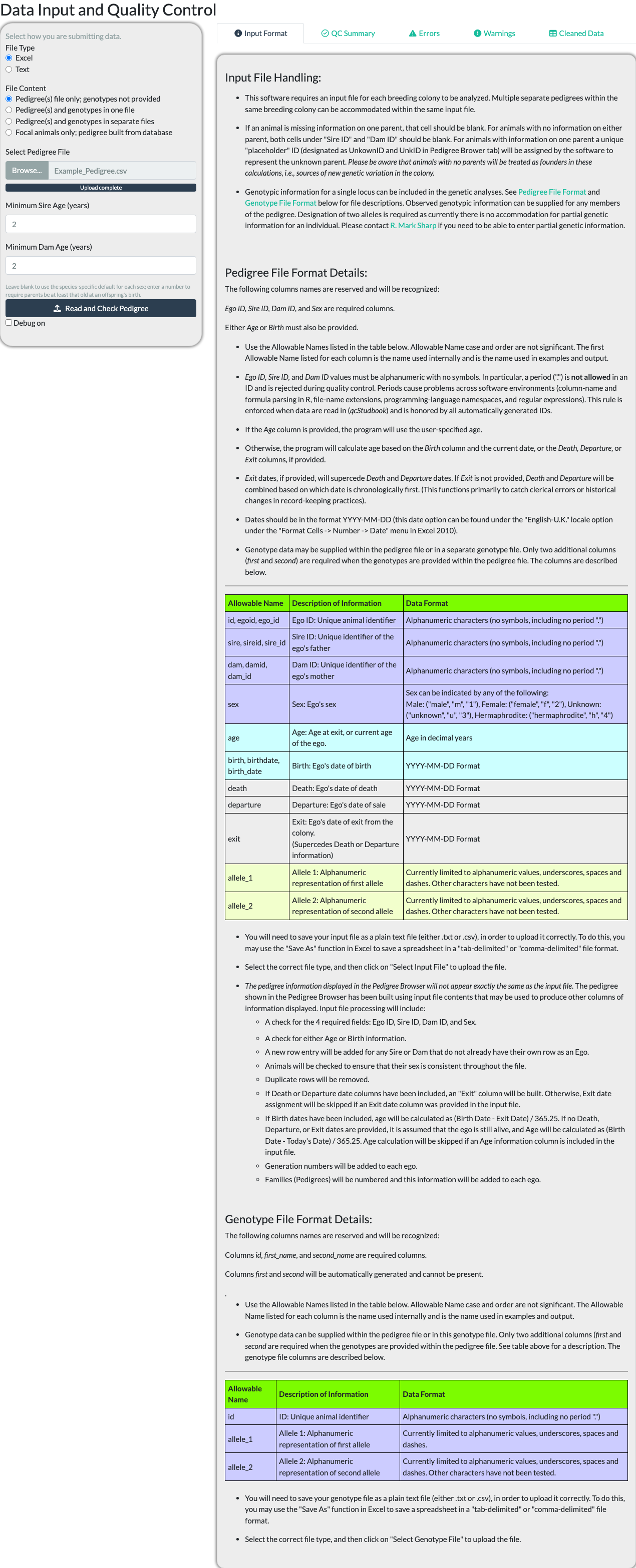
The Japanese macaque example in the package, deidentified_jmac_ped.csv, shows why this matters: 62 of its mothers were between 3.38 and 3.99 years old at a birth, under the built-in 4-year floor for Japanese macaque females, and 13 of its fathers were as young as 4.36, under the 5-year floor for males, so the file loads only once Minimum Dam Age is set to 3.3 or lower and Minimum Sire Age to 4.3 or lower.
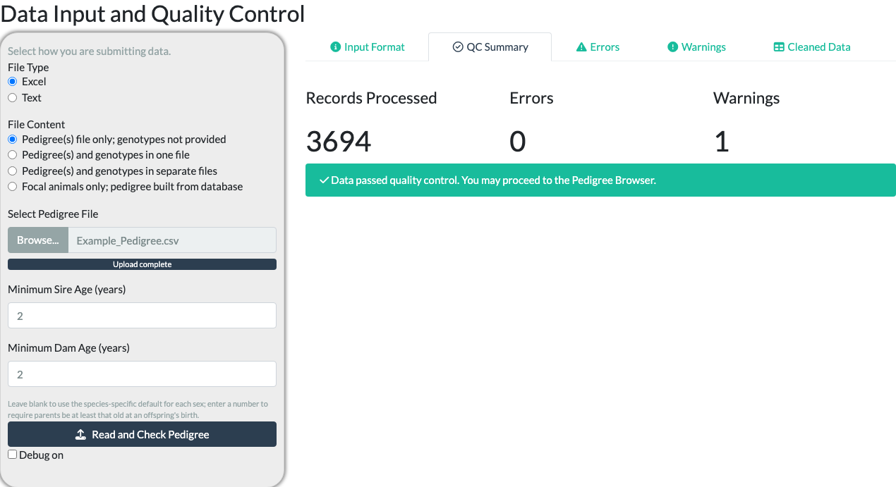
Selecting Read and Check Pedigree reads the file and validates it – checking that every required column is present and that the pedigree is internally consistent (parent-of-the-right-sex, no duplicate IDs, valid dates, and more; the full set of checks is listed below). The counts are on the “QC Summary” sub-tab, the second of the five sub-tabs along the top of the results (“Input Format”, “QC Summary”, “Errors”, “Warnings” and “Cleaned Data”). Each count box is colored by what the check found: Records Processed is always dark blue; Errors is red when there is at least one error and green when there are none; Warnings is orange when there is at least one warning and green when there are none. When the check finds errors, the app opens the “Errors” sub-tab for you and shows a red notice in the lower right corner, “QC found N error(s). Check the Errors tab.” (N is the number of errors); when it finds only warnings, it opens the “Warnings” sub-tab and shows a yellow notice, “QC found 2 warning(s). Check the Warnings tab.” (here 2 is the number of warnings). The notice closes by itself after a few seconds, and the sub-tab it names is already open; you click “QC Summary” for the counts. For the shipped example pedigree read as CSV, the counts are Records Processed: 3,694, Errors: 0, Warnings: 2. The first warning, “Column name case changed”, names the two columns (recordStatus and fromCenter) whose names were changed to lowercase. The second, “Animals with no birth date”, says that 1,432 of the 3,694 animals (all of them founders) have no birth date, so their age is unknown and the age-based checks and counts – the parent-age check, the Age-Sex Pyramid and the breeding-age counts – cannot use them. Another warning, “Animals with a death or departure before birth”, appears only when a file has animals whose death or departure date is earlier than their birth date: it says how many, names the first five, and notes that their age comes out zero or negative. The shipped example has none, and a death or departure on the birth day is not flagged. A warning never stops the pedigree from being used.
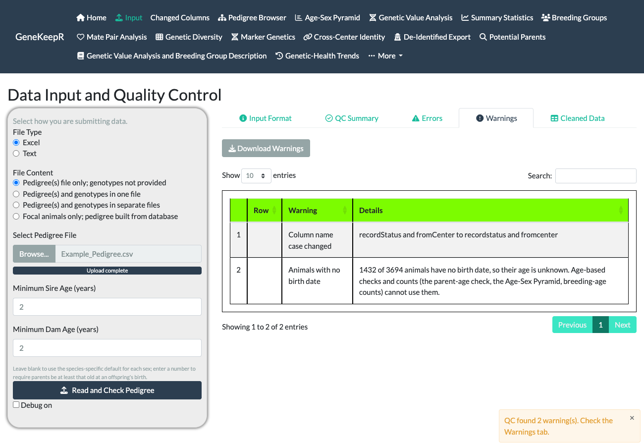
The picture below shows the Warnings sub-tab as the app opens it for this file: one row for each of the two warnings, with the yellow notice still on screen in the lower right corner.
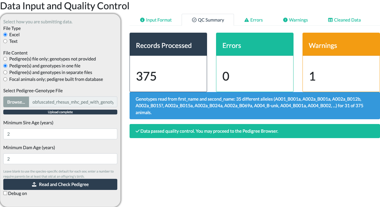
In “Pedigree(s) and genotypes in one file” mode the QC Summary adds one line under the three boxes, saying which columns were read, how many different alleles it found and for how many animals: a line beginning “Genotypes read from” or, when no usable pair of columns was found, one beginning “No genotype columns were found” that names the column names it looked for, or one beginning “Genotype columns were found” that names the columns that are not a usable pair. Check the number of alleles: a misspelled label counts as one more. The picture below reads the package’s shipped file obfuscated_rhesus_mhc_ped_with_genotypes.csv (found with system.file("extdata", "examples", "obfuscated_rhesus_mhc_ped_with_genotypes.csv", package = "nprcgenekeepr")), the rhesus MHC example pedigree of 375 animals with the genotype labels of its 31 genotyped animals in first_name and second_name: 35 different alleles for 31 of the 375 animals. The one warning is unrelated to the genotypes: 85 of the 375 animals have no birth date.
| Error | Definition |
|---|---|
| failedDatabaseConnection | Database connection failed: configuration or permissions are invalid. |
| missingColumns | Columns that must be within the pedigree file are missing. |
| invalidDateRows | Values that are supposed to be dates cannot be interpreted as a date. |
| suspiciousParents | A parent was too young, on the offspring’s birth date, to plausibly be the parent. |
| femaleSires | Individuals listed as female or hermaphroditic and also as a sire. |
| maleDams | Individuals listed as male and also as a dam. |
| sireAndDam | Individuals listed as both a sire and a dam. |
| duplicateIds | IDs listed more than once. |
| invalidIdChars | IDs (id, sire, or dam) containing a disallowed period (‘.’); IDs must be alphanumeric with no symbols. |
| invalidPlaceholderRows | Values in an optional placeholder column (TRUE or FALSE, marking stand-in unknown parents) other than TRUE, FALSE, 1, 0 or blank. |
| changedCols | Columns renamed to conform to internal naming conventions, and what they were changed to. |
Pedigree Browser
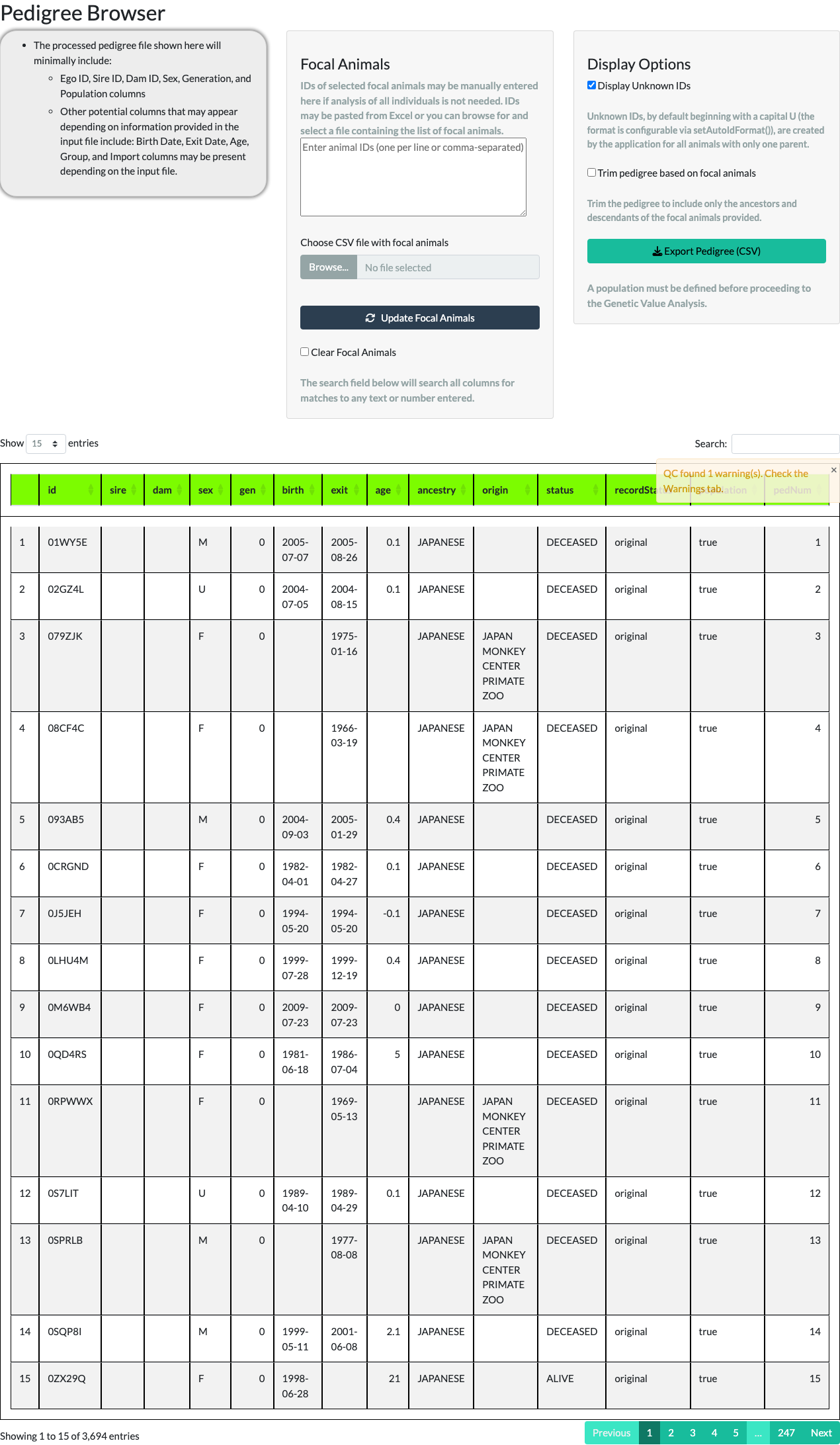
The Pedigree Browser tab displays the pedigree in a paged table (15 rows at a time by default, adjustable) with a Display Unknown IDs option. Unknown IDs (UIDs) are placeholder IDs the application generates, by default starting with the letter U, for the unrecorded parent of an animal with only one known parent.
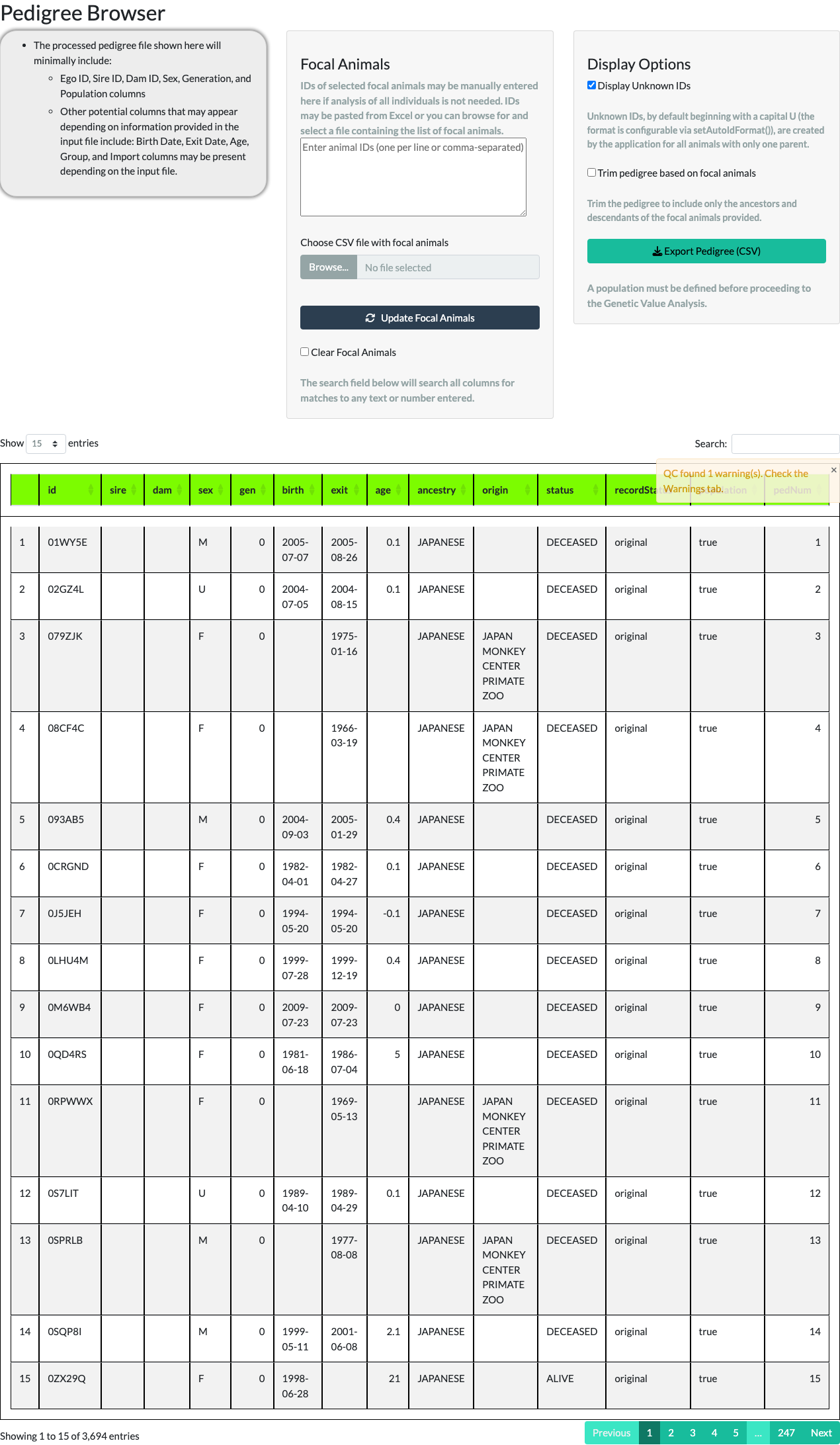
Which rows are placeholders is recorded in a yes/no placeholder column that the quality check adds (TRUE for a made-up parent, FALSE for a real animal). If a real animal’s ID looks like a made-up one, such as U1234, enter FALSE for it in that column of your file and it stays visible. The column is kept in the files you download, so the marks survive a save and re-upload.
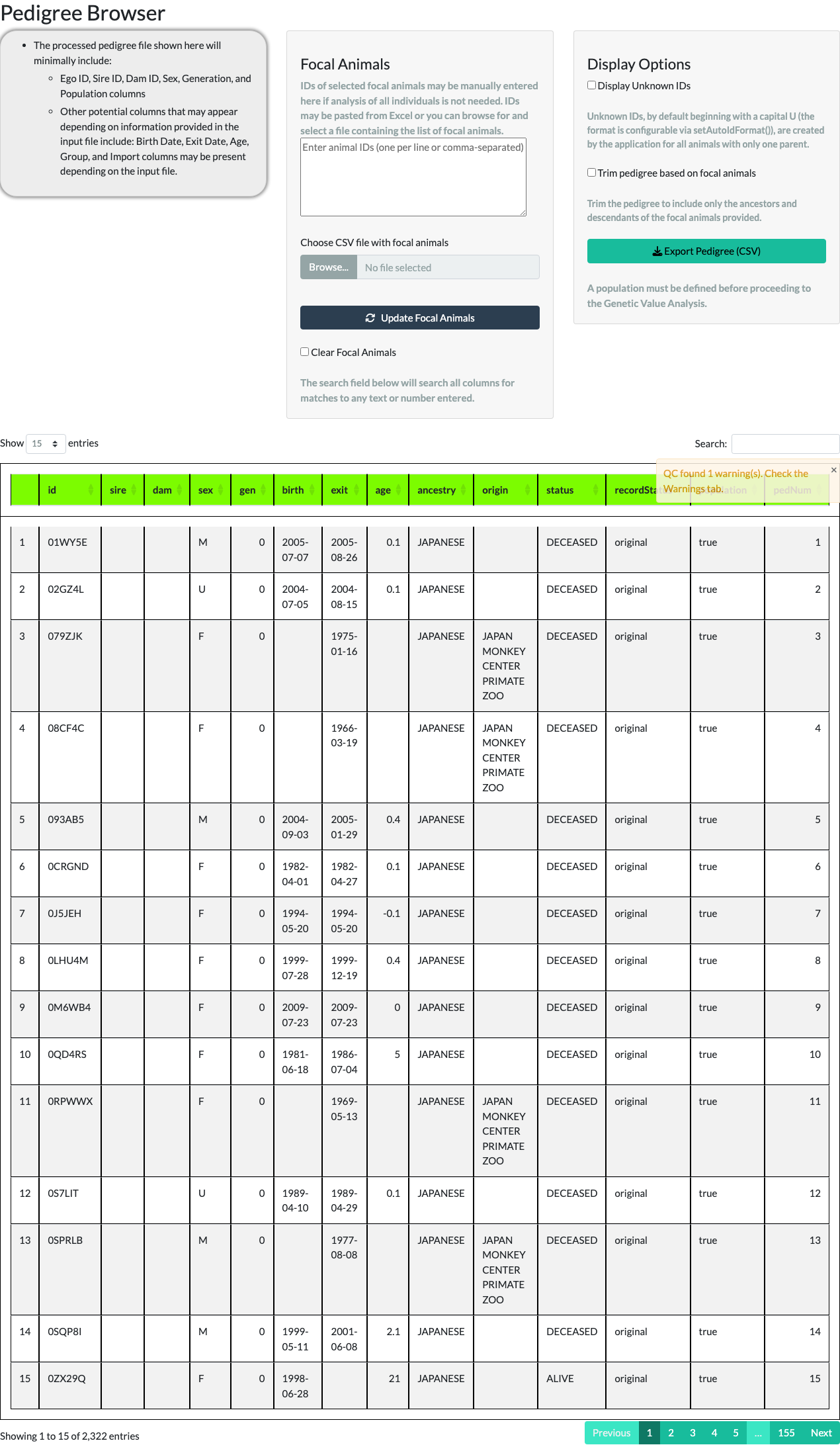
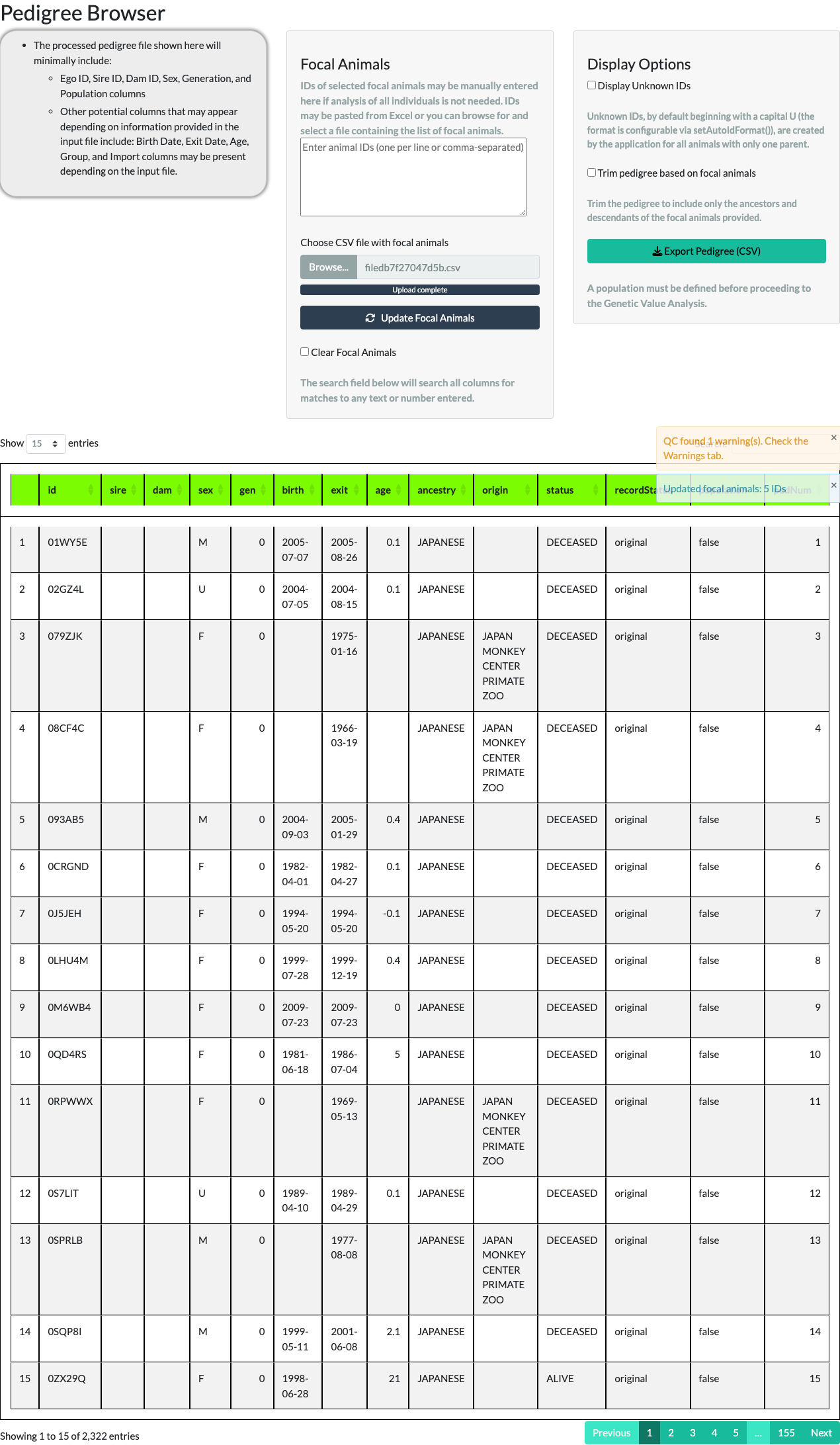
Unchecking Display Unknown IDs removes those placeholder rows. For the example pedigree, the row count reduces from 3,694 to 2,322 – the difference, 1,372, is the number of UNKNOWN placeholder animals the application generated to stand in for unrecorded parents. The box changes only this table: the other tabs, such as Genetic Value Analysis, still use every animal, so unchecking it never breaks an analysis.
Focal animals. The middle panel lets you narrow the browser to a subset of the pedigree – your focal animals – either by typing IDs directly or by uploading a CSV file of IDs.
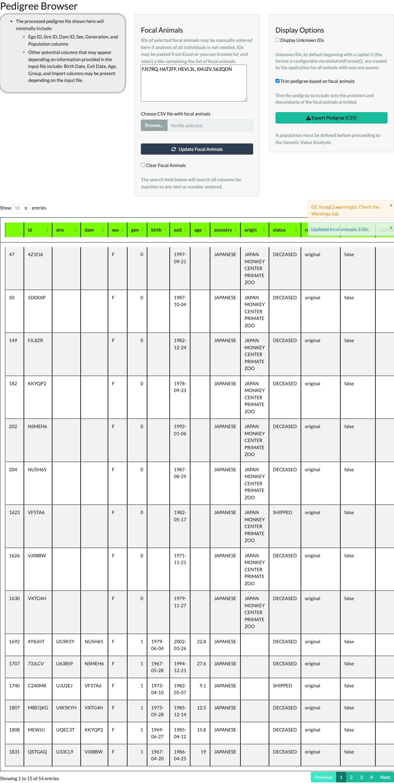
Typing five IDs (FJS7RQ, H6T2FF, HEVL3L, I04JZV, S63QDN), unchecking Display Unknown IDs, checking Trim pedigree based on focal animals, and selecting Update Focal Animals keeps only those five animals and their ancestors and descendants – 54 animals in total for this example.
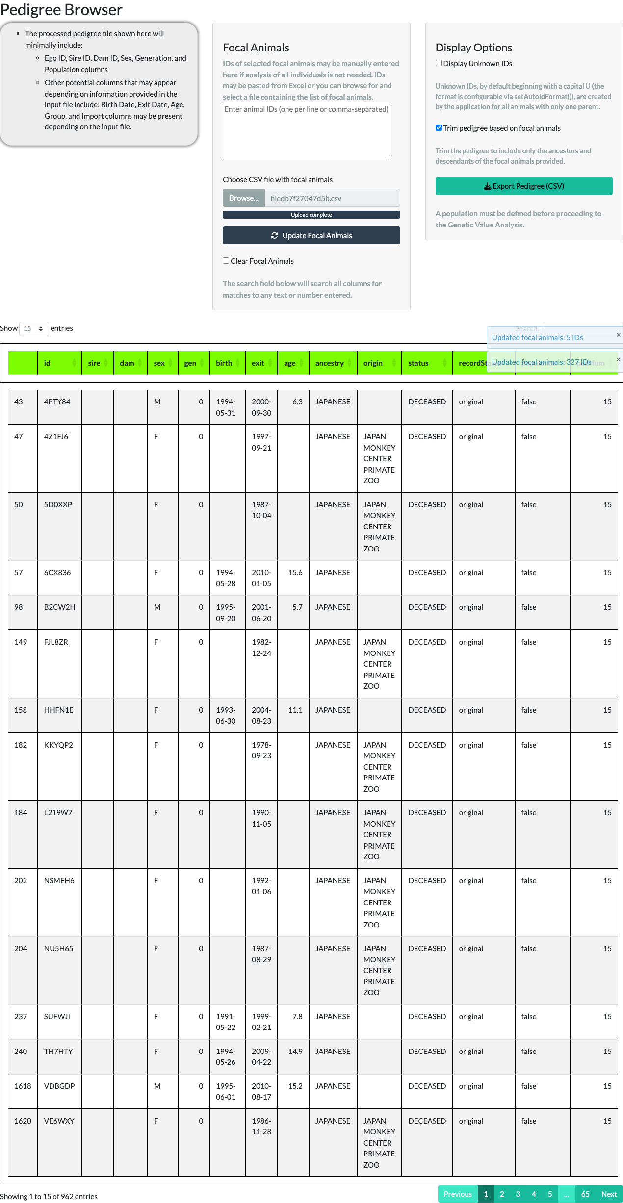
A larger focal-animal list works the same way. The package ships a second example object, data(focalAnimals), with 327 IDs; uploading it as a CSV via Choose CSV file with focal animals and trimming keeps those animals plus everyone needed to connect them – 962 animals in total.
focalAnimals example, 327 IDs).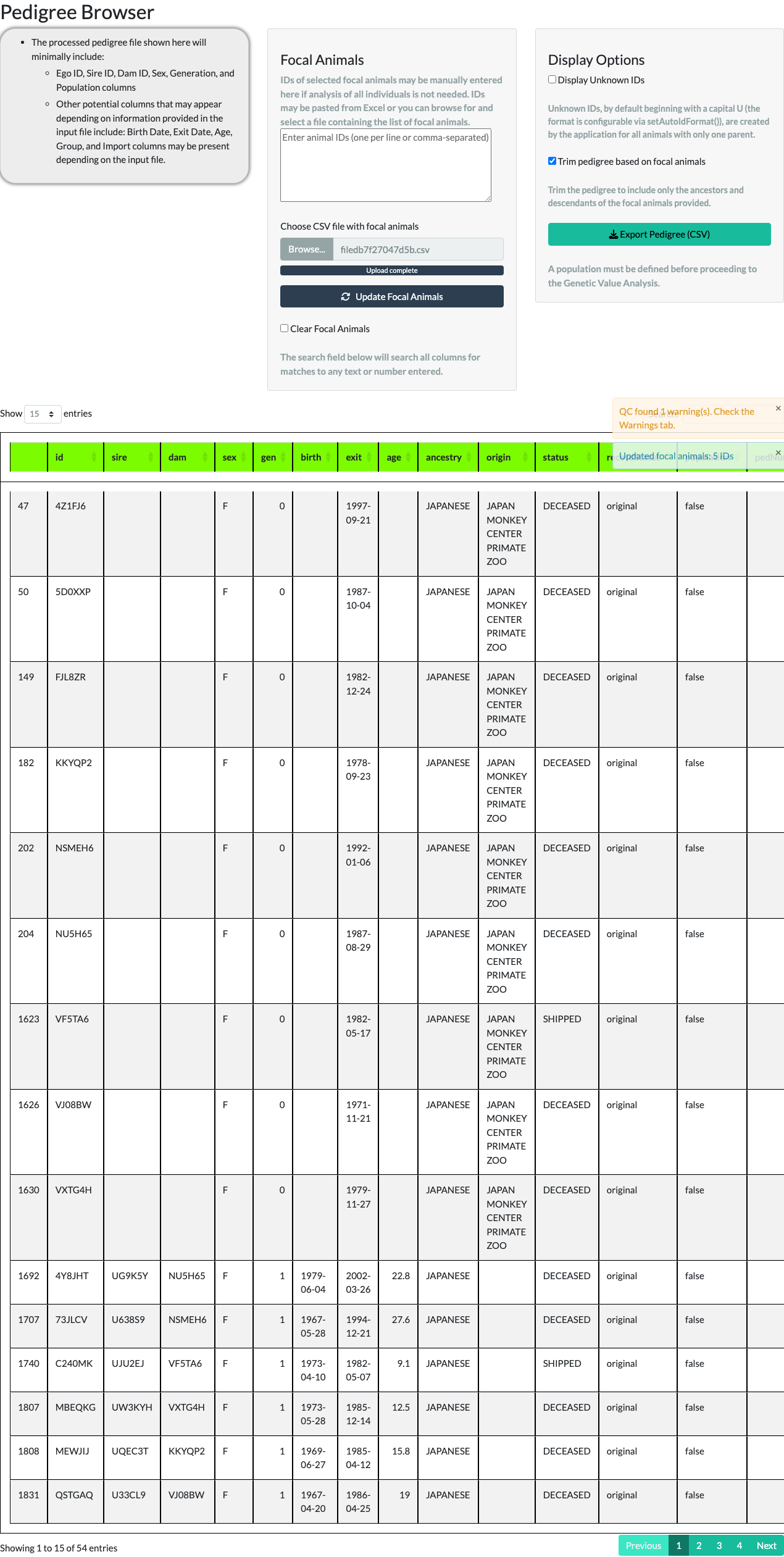
Checking Clear Focal Animals and selecting Update Focal Animals again reads an empty ID list, restoring the full, untrimmed pedigree and making the living animals the population again.
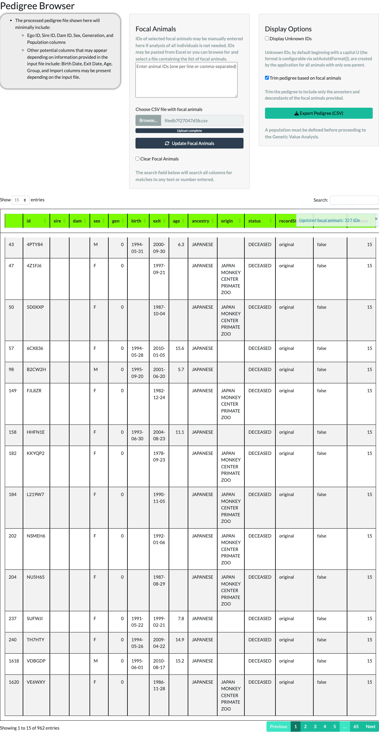
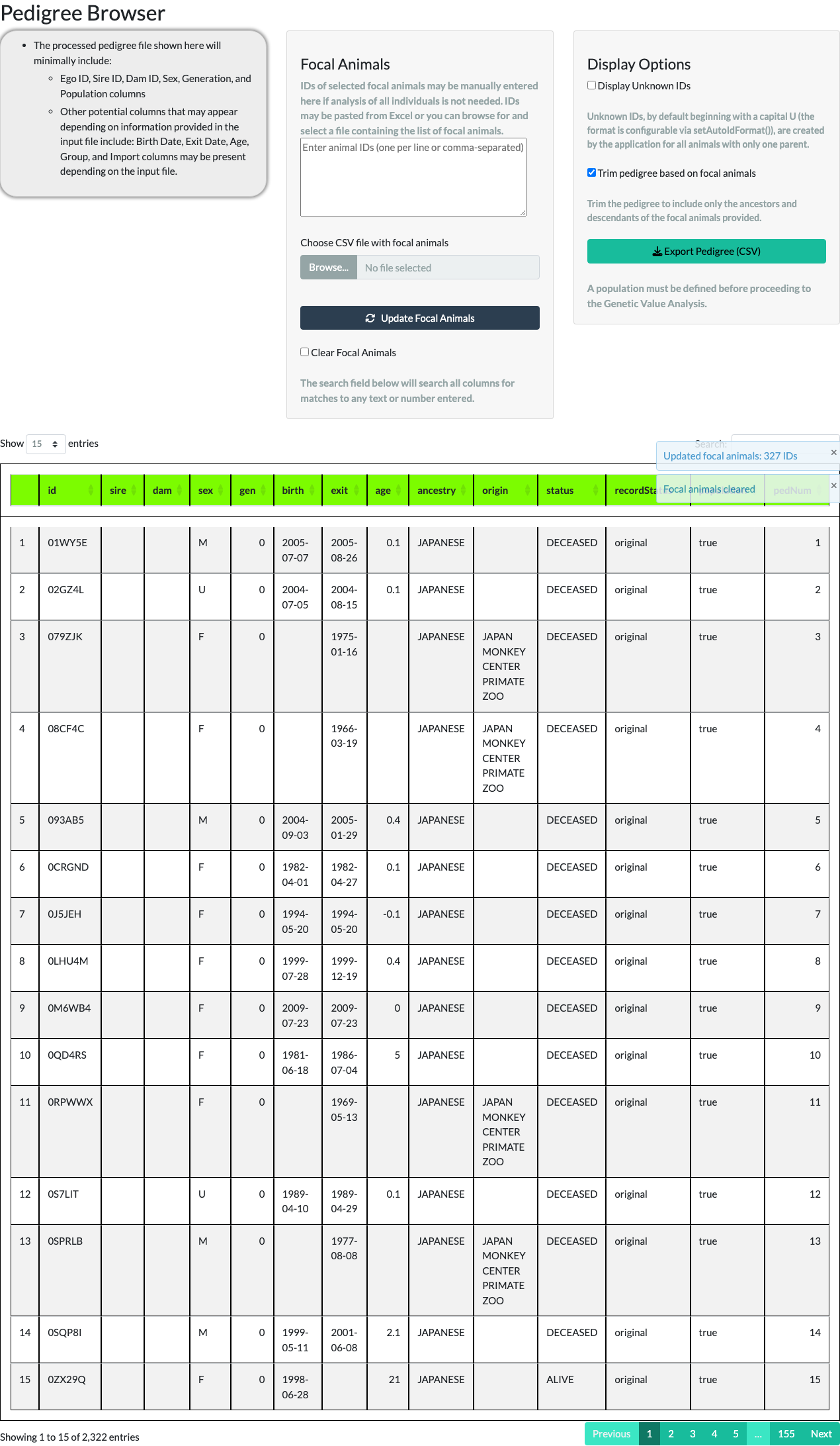
With no focal animals entered, the population the other tabs analyze is the living animals (every animal if none is alive). The rest of this walkthrough continues with the full, untrimmed example pedigree and no focal animals, so its population is the 332 living animals (the focal-animal trim above illustrates the feature, not the population used for the remaining tabs) – matching the shipped examplePedigree’s own downstream numbers below.
Diagram view. Alongside the table, the Pedigree Browser’s Diagram tab renders the same population as an interactive pedigree diagram: one node per animal, shaped by sex, connected via a mating-unit convention – a mate’s own matings render as a small connector between the two parents, with a line down to their shared children, the same convention traditional pedigree charts (and the kinship2 R package) use. A Diagram Edge Style toggle above the diagram switches between a strict-right-angle routing matching kinship2’s own look (the default) and a straight-line routing. A legend to the right of the diagram shows what each shape means. If the pedigree data includes an optional affected column, individuals marked affected are additionally shaded a distinct color, with a matching “Affected” entry in the same legend – pedigrees without an affected column render unshaded, as before. If the pedigree data includes an optional name column, a Show Names on Diagram toggle above the diagram (off by default) switches each node’s label from id-only to id plus name on a second line – a name longer than 15 characters is truncated with an ellipsis on the diagram itself, with the full name always available in the hover tooltip. Not every animal needs a name; one with no name, or a pedigree with no name column at all, always renders with just its id, and the “Select by id” search dropdown below always lists ids, never names, regardless of the toggle. A mating between two blood-related animals renders its connector lines thicker and in a distinct color, flagging the consanguineous mating at a glance – no optional column or toggle needed, since it is detected directly from the pedigree’s own sire/dam data. If a colony records twin births, an optional Twin/Zygosity Relations file can be uploaded to draw a distinctly-styled connector between a declared pair’s own nodes – and, for a declared monozygotic pair, corrects their kinship to genetic identity throughout the application, not just this diagram. See The Pedigree Diagram Tab article for the full tour of every feature this tab offers, with a screenshot of each.
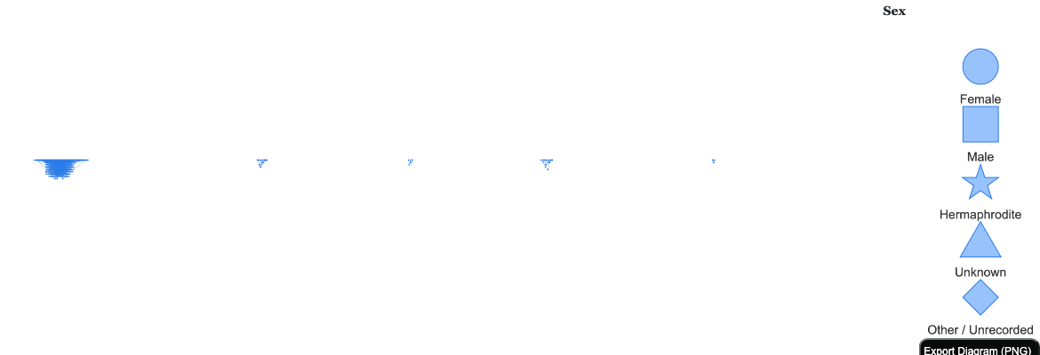
Diagrams render up to 400 animals under the default rectilinear style (750 if switched to the straight-line style) – for larger populations, narrow the focal-animal selection first (see Focal animals above). Hovering any node shows its ID, sex, generation, sire, dam, and (when present) affected status without leaving the diagram. Clicking a node re-centers the population on that animal, the same as typing its ID into the focal-animals text area above – a quick way to explore a different branch of the pedigree. A Select by id dropdown above the diagram lets you jump straight to one animal by ID, dimming every other node except it and its direct connections – useful for finding one animal in a large, busy diagram. An Export Diagram (PNG) button in the diagram’s own corner saves the current view as an image file, useful for husbandry reports, IACUC documents, or presentations.
Age-Sex Pyramid
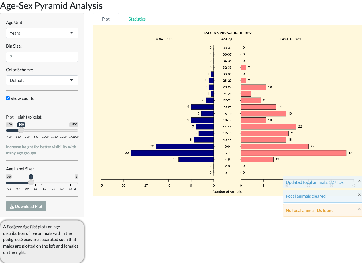
The Age-Sex Pyramid tab displays a standard population pyramid for whichever pedigree population is currently selected in Pedigree Browser, with options for age units, color scheme, and whether to show counts. For the full example pedigree, it shows 332 living animals (123 male, 209 female).
Genetic Value Analysis
The Genetic Value Analysis tab ranks animals by relative breeding value, using mean kinship (how inter-related an animal is with the rest of the current breeding population – lower is better) and genome uniqueness (how likely an animal carries alleles that are rare in the colony and at risk of being lost – higher is better). See the Genetic Value Analysis and Breeding Group Description tab for the full calculation breakdown.
Genome uniqueness is estimated by a gene-drop simulation (MacCluer et al. 1986; Ballou and Lacy 1995): unique alleles are assigned to every pedigree founder and simulated forward through the pedigree according to Mendelian rules. Because it is an estimate, each value carries a sampling standard error (the guSE column) that shrinks roughly with the square root of the iteration count – but what actually matters for breeding decisions is whether the ranking order has stabilized, not just whether guSE is small. The default is 1,000 iterations, which experience with the pedigrees this package has been used on gives a stable selection order; to check whether 1,000 is enough for a specific pedigree, run gvaConvergence() (see the Gene-Drop Iteration Convergence vignette, vignette("gvaConvergence", package = "nprcgenekeepr")).
An optional Kinship Overrides panel accepts a CSV or Excel file of outside-information kinship values (columns id1, id2, kinship) for specific pairs – for example, genotype-confirmed relatedness that disagrees with the pedigree. Overrides apply to rankings, breeding groups, and summary statistics regardless of tab order, though the Summary Statistics relationship label stays pedigree-derived even when its displayed value is overridden.
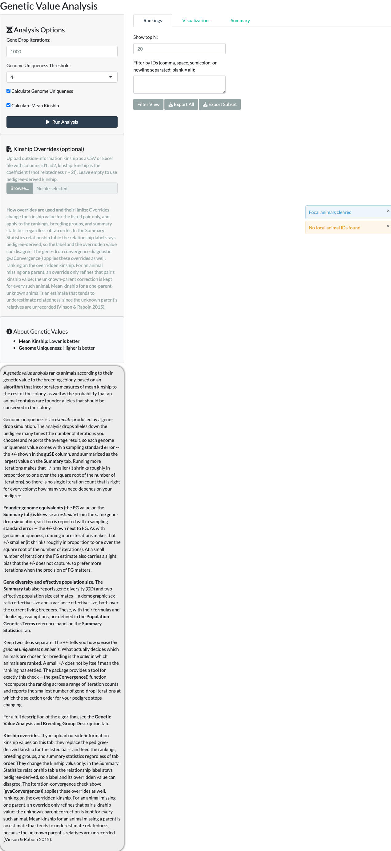
Selecting Run Analysis starts the gene-drop process. When it completes, a results table shows each animal’s rank, mean kinship, genome uniqueness, and a value column classifying it as High Value, Low Value, or Undetermined. “Show top N” and an ID filter control how many rows are displayed.
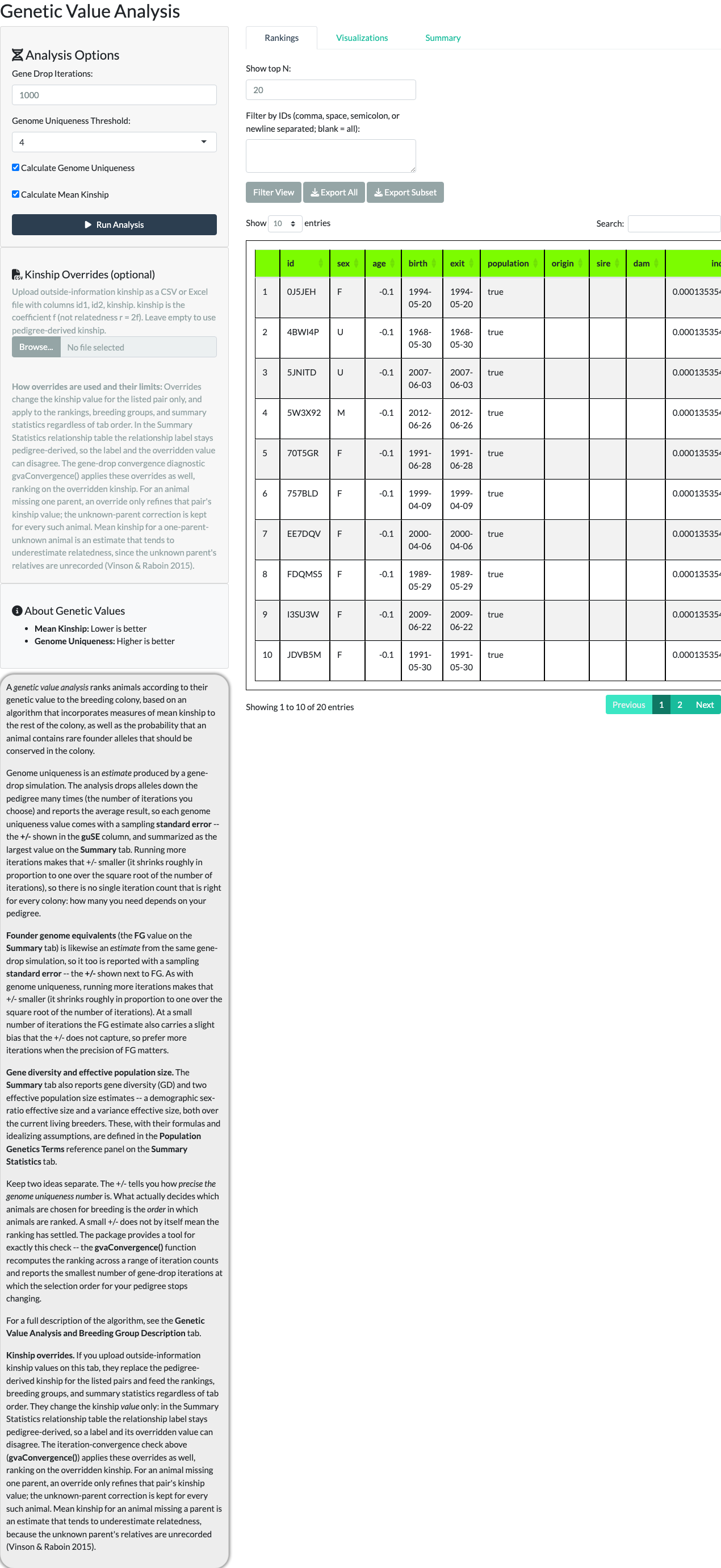
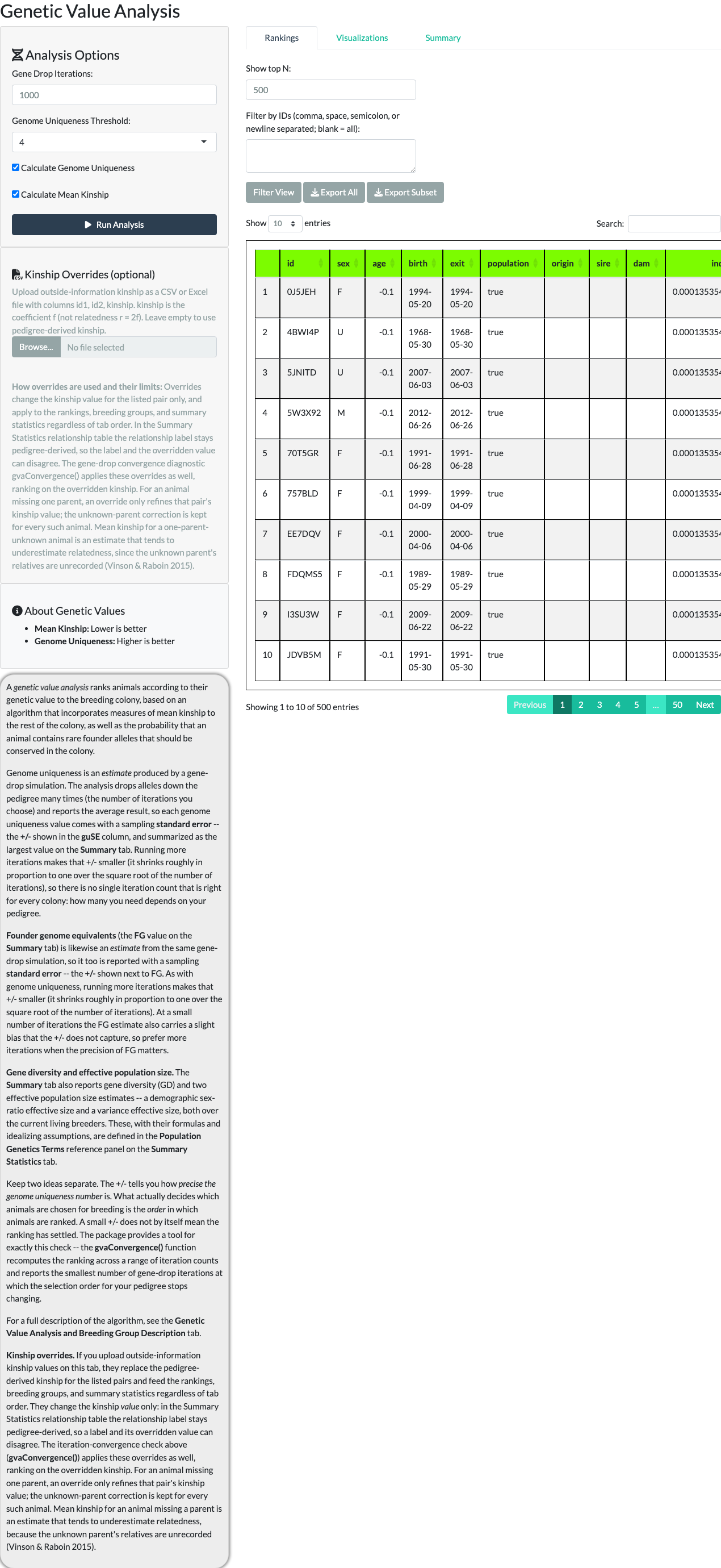
A correction to an older claim. Animals with no recorded parentage (“Undetermined”: both parents unknown and no recorded origin; animals that are genuine imports, with a recorded origin, are ranked normally) are not automatically high value. Since issue #9’s ranking correction (the Undetermined demotion in R/modGeneticValue.R), the results table sorts Undetermined animals to the bottom of the ranking, so a genuinely uncertain genome-uniqueness estimate no longer inflates them to the top. Because the exact row at which values transition from High to Low is a property of one stochastic gene-drop run, this article does not pin a specific row number to it – widening “Show top N” (to 500 below) shows the full distribution instead.
Summary Statistics
The Summary Statistics and Plots tab uses the results from Genetic Value Analysis. Definitions of genome uniqueness and kinship are on the Genetic Value Analysis and Breeding Group Description tab; founder-equivalent and founder-genome-equivalent definitions are at the bottom of this tab (see also “Validating the Founder-Genome-Equivalent Standard Error”).
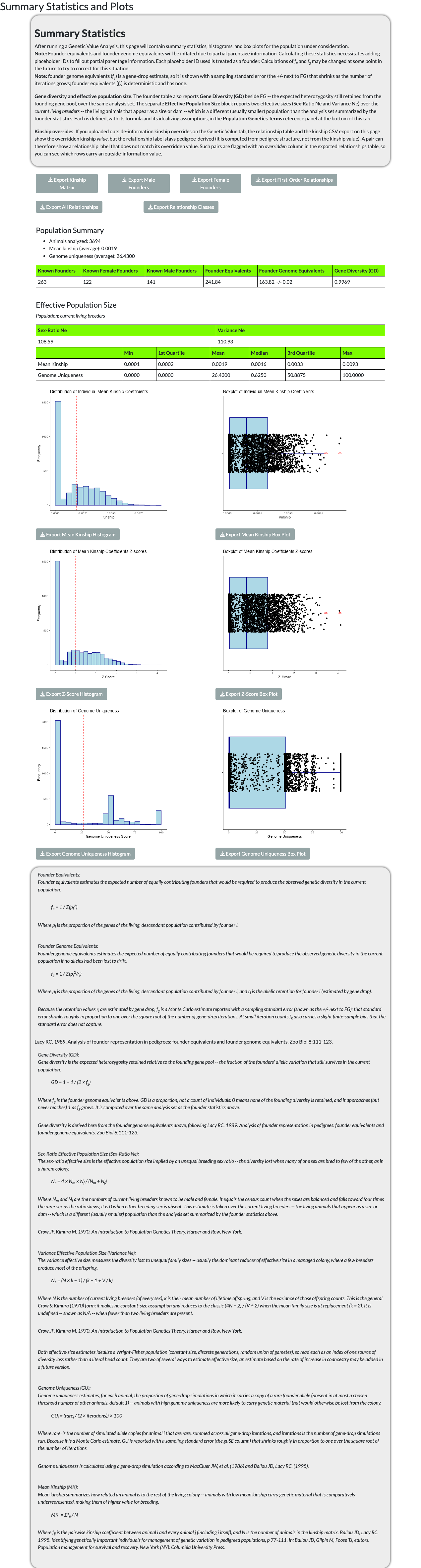
The tab has several export buttons producing CSV files, three of which are shown below: Export Kinship Matrix, Export First-Order Relationships, and Export Female Founders (a separate Export Male Founders button produces the same column structure for males). These tables are not screenshots. This article builds them each time it is rendered, from the example pedigree and the same package functions the export buttons call, and shows each file’s own contents (NA marks a blank value). The tab also has Export All Relationships and Export Relationship Classes buttons, plus six further buttons for exporting the six summary plots below as PNGs, not illustrated here:
Kinship matrix. The file has a row and column for every analyzed individual, plus a first row and first column of IDs. Most pairs of animals are unrelated and show 0, so the table below shows only a corner: the first animal with three or more offspring (0ZX29Q) and its first three offspring, where the values are not zero.
| 0ZX29Q | D9MZ4A | LVXPH7 | NF8IQG | |
|---|---|---|---|---|
| 0ZX29Q | 0.5 | 0.25 | 0.25 | 0.25 |
| D9MZ4A | 0.25 | 0.5 | 0.125 | 0.125 |
| LVXPH7 | 0.25 | 0.125 | 0.5 | 0.125 |
| NF8IQG | 0.25 | 0.125 | 0.125 | 0.5 |
First-order relationships. The file has columns id, parents, offspring, siblings, and total, counted from known relationships, one row per animal.
| id | parents | offspring | siblings | total |
|---|---|---|---|---|
| 01WY5E | 0 | 0 | 0 | 0 |
| 02GZ4L | 0 | 0 | 0 | 0 |
| 079ZJK | 0 | 2 | 0 | 2 |
| 08CF4C | 0 | 1 | 0 | 1 |
| 093AB5 | 0 | 0 | 0 | 0 |
| 0CRGND | 0 | 0 | 0 | 0 |
| 0J5JEH | 0 | 0 | 0 | 0 |
| 0LHU4M | 0 | 0 | 0 | 0 |
Founders. The founders files have columns id, sire, dam, sex, gen, birth, exit, age, ancestry, origin, status, recordStatus, fromCenter, placeholder, population, and pedNum. The table scrolls sideways to show every column.
| id | sire | dam | sex | gen | birth | exit | age | ancestry | origin | status | recordStatus | fromCenter | placeholder | population | pedNum |
|---|---|---|---|---|---|---|---|---|---|---|---|---|---|---|---|
| 079ZJK | NA | NA | F | 0 | NA | 1975-01-16 | NA | JAPANESE | JAPAN MONKEY CENTER PRIMATE ZOO | DECEASED | original | FALSE | FALSE | FALSE | 3 |
| 08CF4C | NA | NA | F | 0 | NA | 1966-03-19 | NA | JAPANESE | JAPAN MONKEY CENTER PRIMATE ZOO | DECEASED | original | FALSE | FALSE | FALSE | 4 |
| 0CRGND | NA | NA | F | 0 | 1982-04-01 | 1982-04-27 | 0.1 | JAPANESE | NA | DECEASED | original | TRUE | FALSE | FALSE | 6 |
| 0J5JEH | NA | NA | F | 0 | 1994-05-20 | 1994-05-20 | -0.1 | JAPANESE | NA | DECEASED | original | TRUE | FALSE | FALSE | 7 |
| 0LHU4M | NA | NA | F | 0 | 1999-07-28 | 1999-12-19 | 0.4 | JAPANESE | NA | DECEASED | original | TRUE | FALSE | FALSE | 8 |
| 0M6WB4 | NA | NA | F | 0 | 2009-07-23 | 2009-07-23 | 0 | JAPANESE | NA | DECEASED | original | TRUE | FALSE | FALSE | 9 |
| 0QD4RS | NA | NA | F | 0 | 1981-06-18 | 1986-07-04 | 5 | JAPANESE | NA | DECEASED | original | TRUE | FALSE | FALSE | 10 |
| 0RPWWX | NA | NA | F | 0 | NA | 1969-05-13 | NA | JAPANESE | JAPAN MONKEY CENTER PRIMATE ZOO | DECEASED | original | FALSE | FALSE | FALSE | 11 |
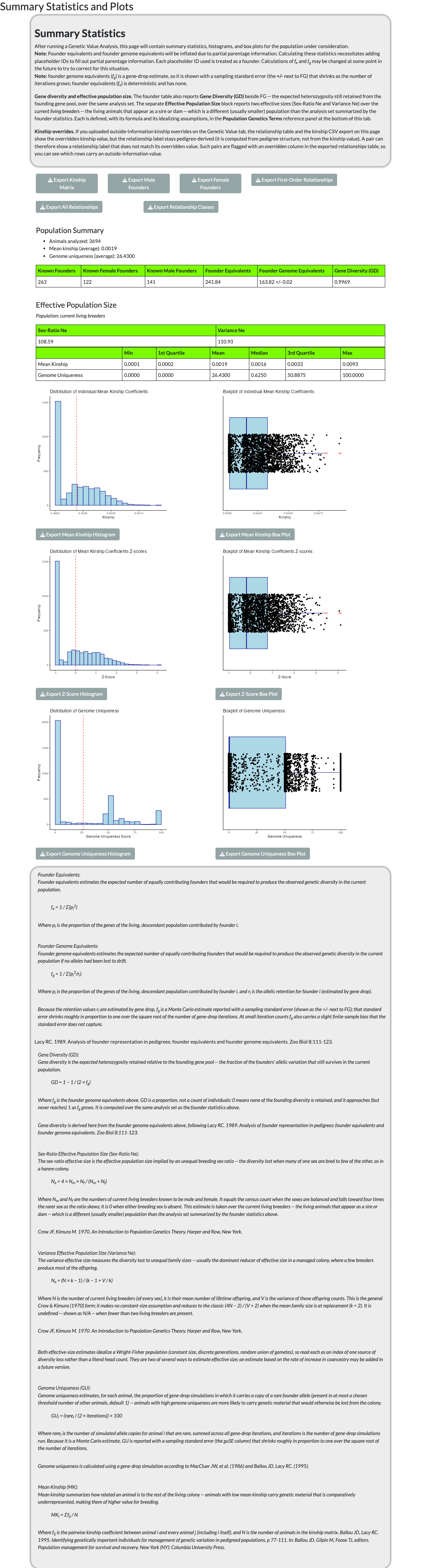
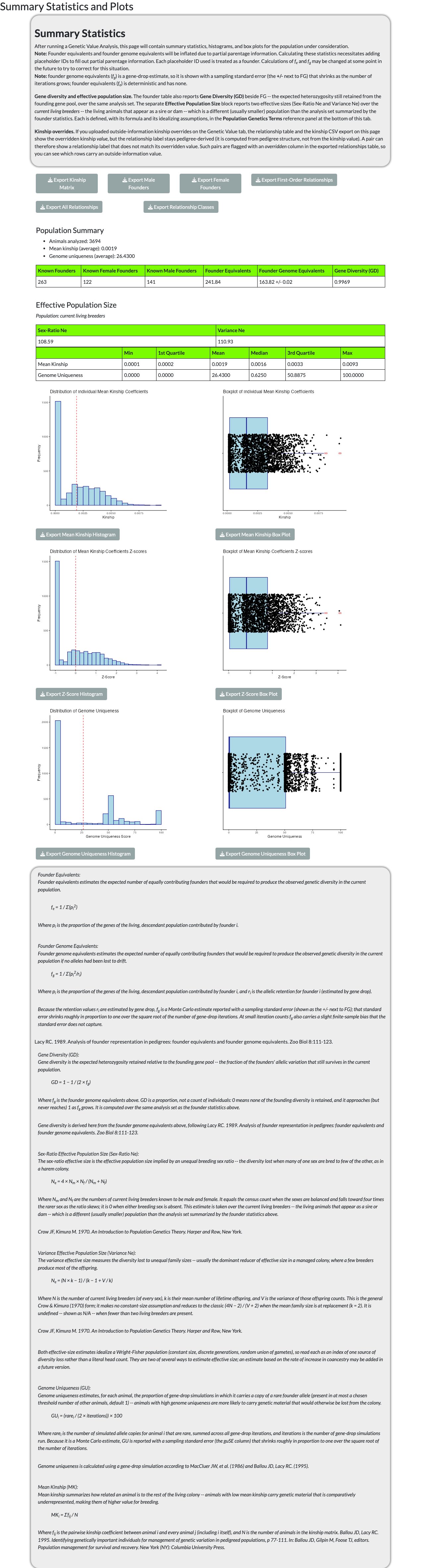
Six plots – histograms and boxplots of kinship coefficients, their Z-scores, and genome uniqueness scores – are shown together and can each be exported as a PNG.
Breeding Group Formation
The Breeding Groups tab forms candidate breeding groups from a source population you choose (top-ranked animals from Genetic Value Analysis, all available animals, or a list of animal IDs you paste in), subject to a maximum kinship threshold, a target number of groups, and a minimum breeding age. Only living animals are used: an animal counts as alive when its Status is ALIVE (or, in a pedigree with no Status column, when it has no exit date), so deceased, shipped and placeholder animals are skipped.
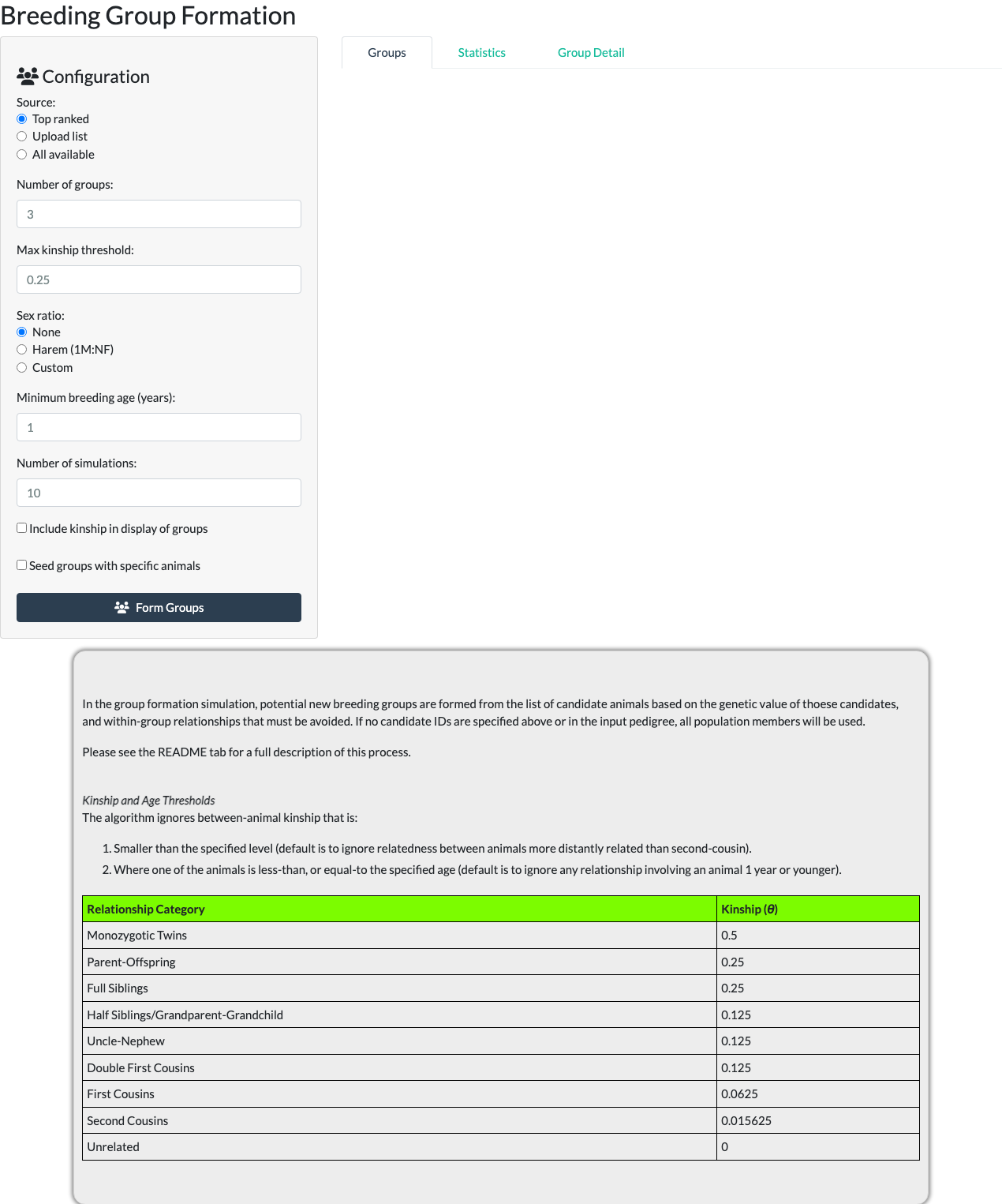
To use only animals you name, choose My own list under Source and paste their IDs into the Animal IDs box that appears.
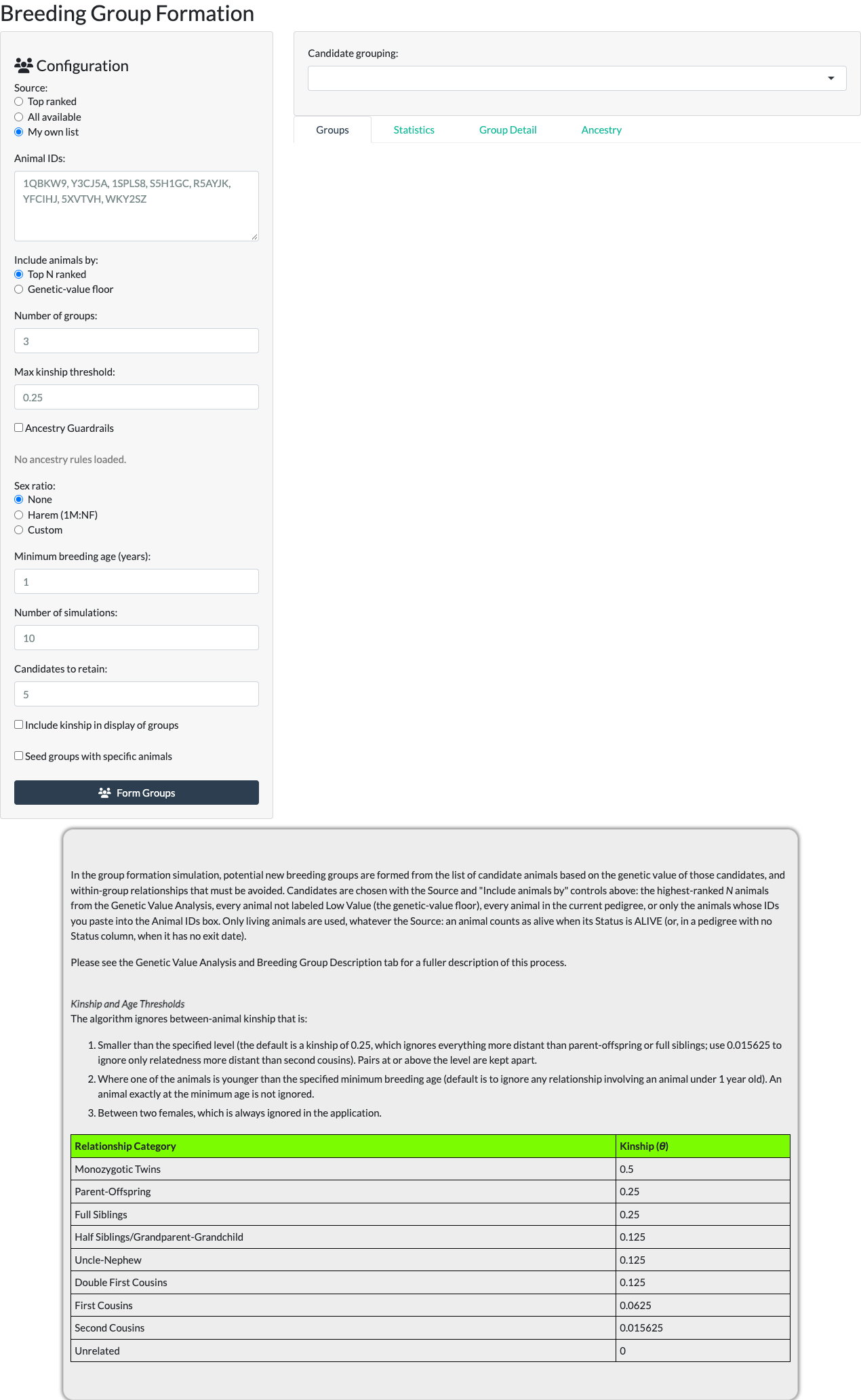
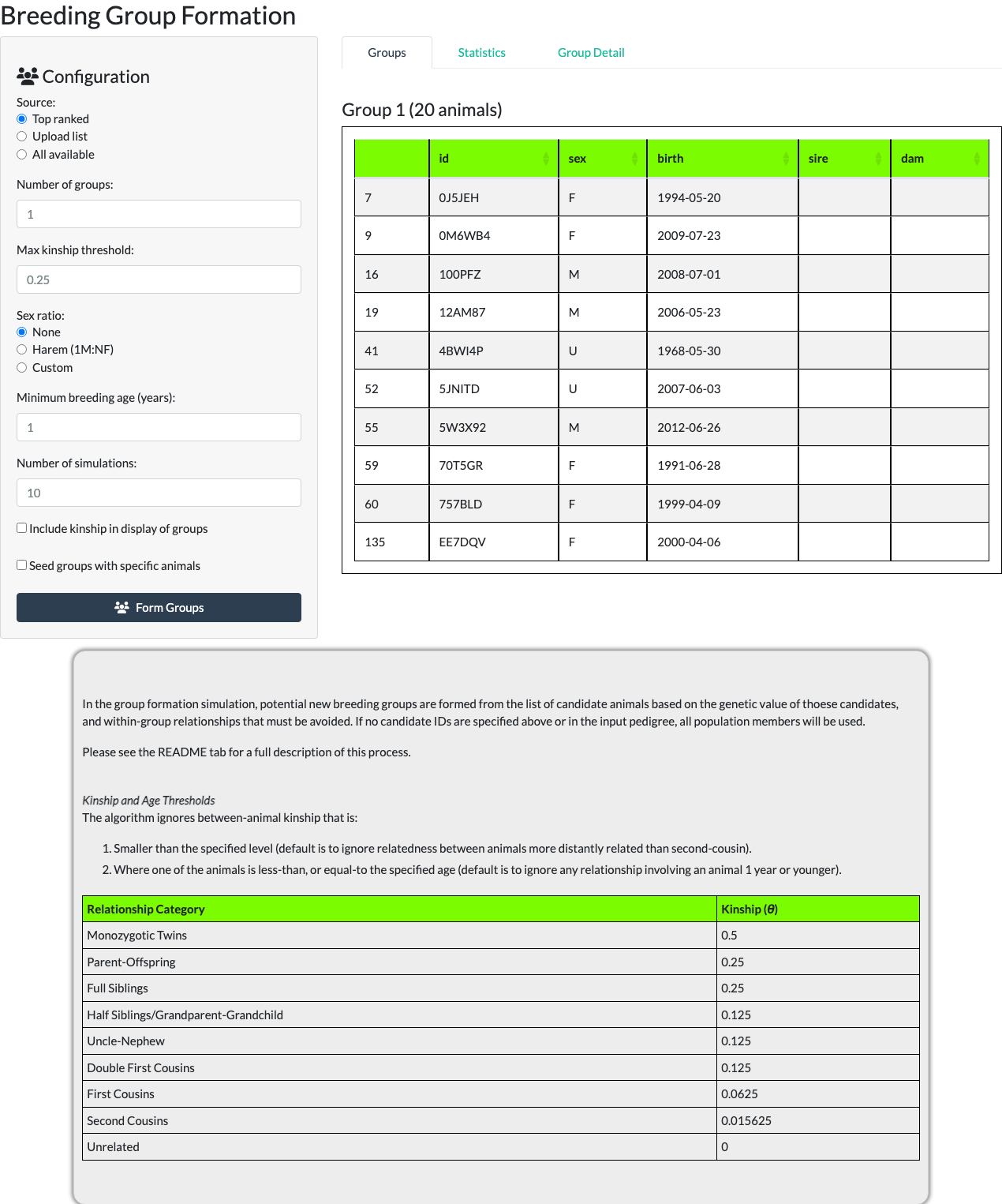
Selecting Form Groups with the number of groups set to 1 produces a single group under the Groups sub-tab.
Sex ratio. Three options control how each group’s sex composition is constrained:
- None – sex is not considered when filling groups.
- Harem (1M:NF) – each group is seeded with a single male and filled with females; as for every other animal, the Max kinship threshold keeps his close relatives out of his group. A male you type into a group’s seed box is that group’s sire; a group whose box holds no male is given one chosen at random.
- Custom – a “Custom ratio (F per M):” numeric field appears (default 1.0, range 0.5-20.0) targeting an arbitrary females-per-male ratio. A male below the Minimum breeding age, or with no birth date, is not placed in any group (he is listed under Unused animals), and a group stops filling when no breeding-age male is left for it, so it can end with fewer females than the ratio asks for.
Note
Fixed before publication. An earlier draft of this walkthrough found selecting “Custom” gave no way to enter the desired ratio anywhere in the UI – internally it was treated the same as “None.” Fixed by adding the numeric field described above; group formation now uses that value as the target ratio.
The screenshot below shows one working example: the default 20 top-ranked candidate animals, a target ratio of 2.5 females per male, and “Number of groups” set to 6. Because group formation is a randomized search (the default Number of simulations is 10), the exact number and composition of groups formed varies from run to run rather than reproducing identically – this particular run produced 6 groups, each drawn toward the target ratio where enough candidates of each sex were available, and a seventh box that lists the seven animals that fit no group.
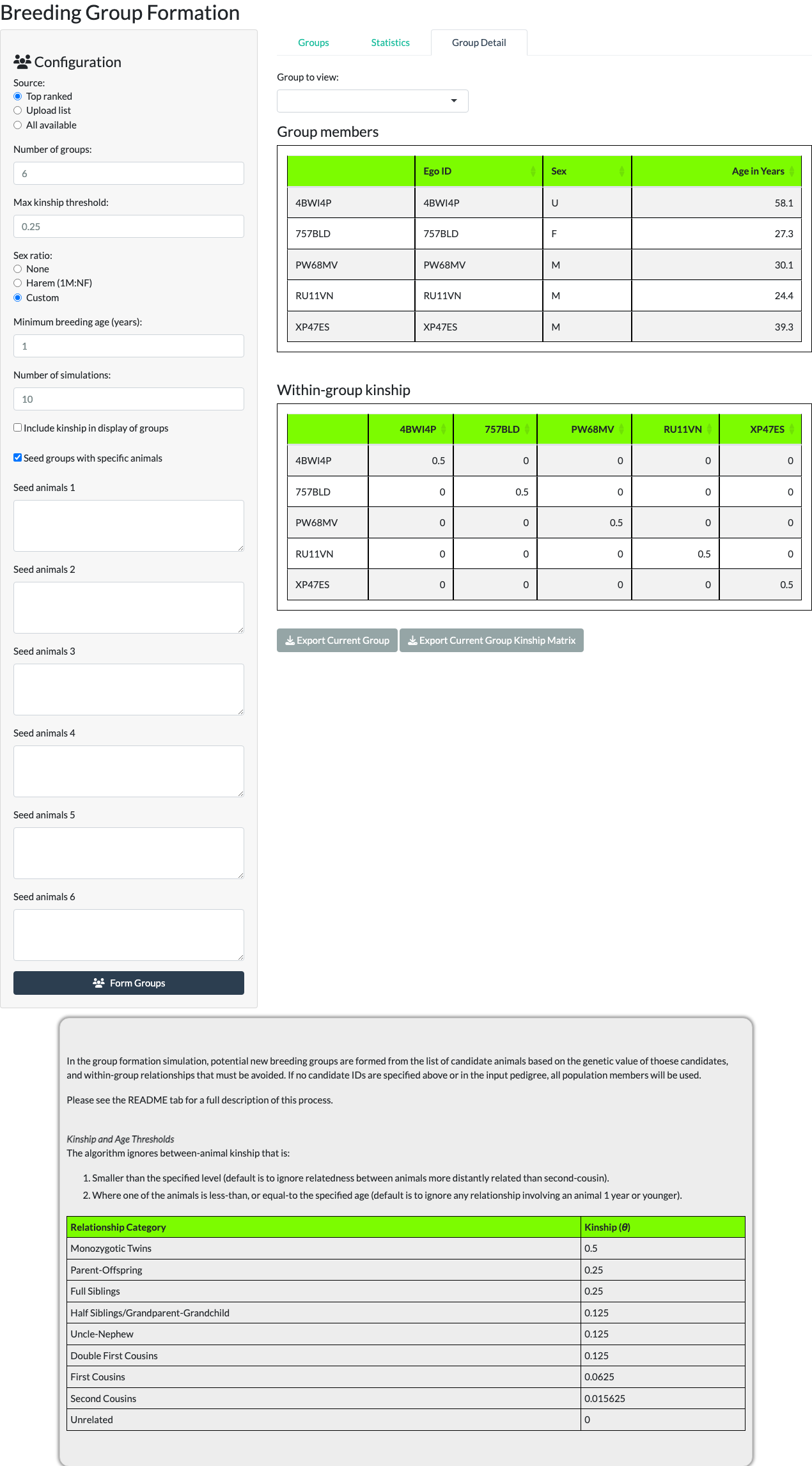
That last box is not a group: it appears only when some candidates fit in no group, and it lists them. The Groups sub-tab, the Statistics table, the Group Detail selector and the Genetic Diversity heat map all call it ‘Unused animals’, and the Groups count in the candidate table above the tabs includes it.
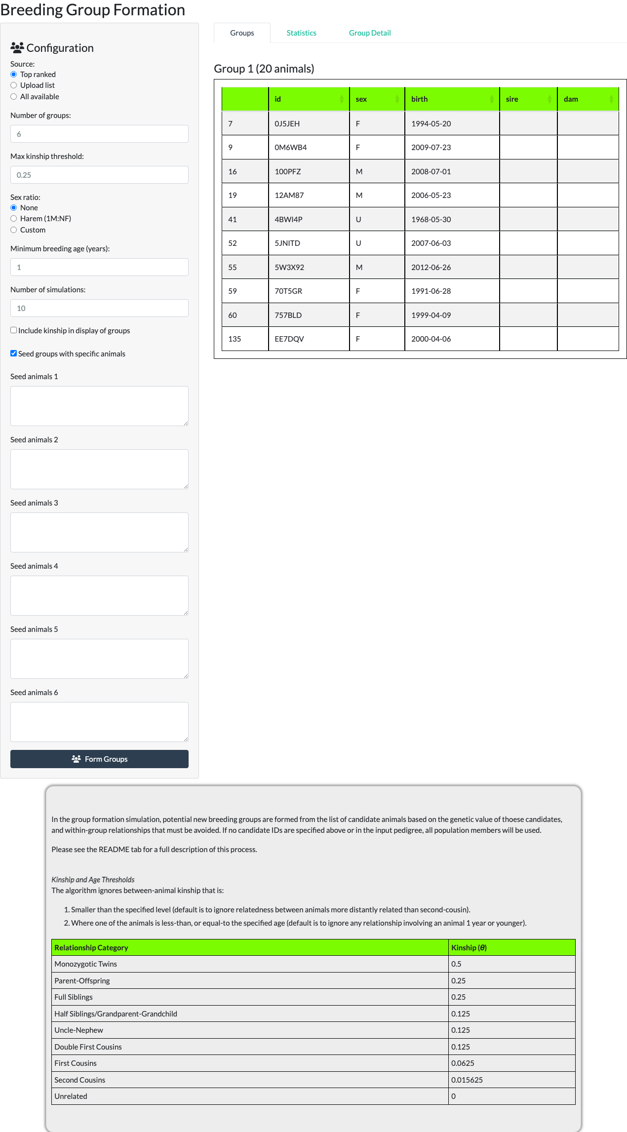
Seeding groups with specific animals. Behavioral constraints – an existing social group, or an infant that should stay with its dam – can be accommodated by checking Seed groups with specific animals, which opens one text area per group for listing the animals that must be assigned to it; the algorithm fills in the remaining membership around those seeds. The screenshot below shows the six text areas this creates for a 6-group run, before any IDs are typed into them.
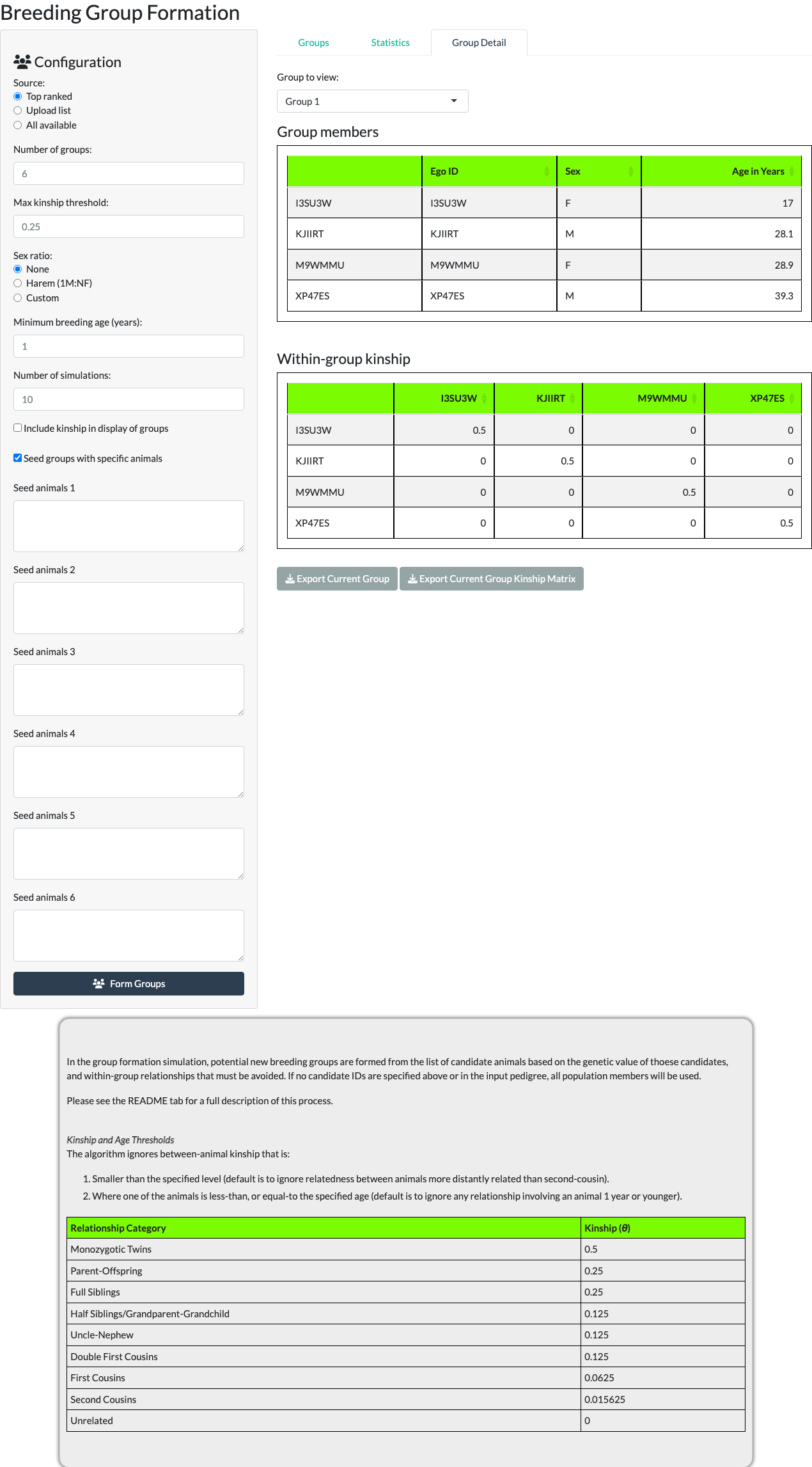
Each formed group’s full membership and its within-group kinship values can be reviewed on the Group Detail sub-tab, one group at a time. The kinship table is shown whether or not Include kinship in display of groups is checked; the box does not change what this sub-tab shows.
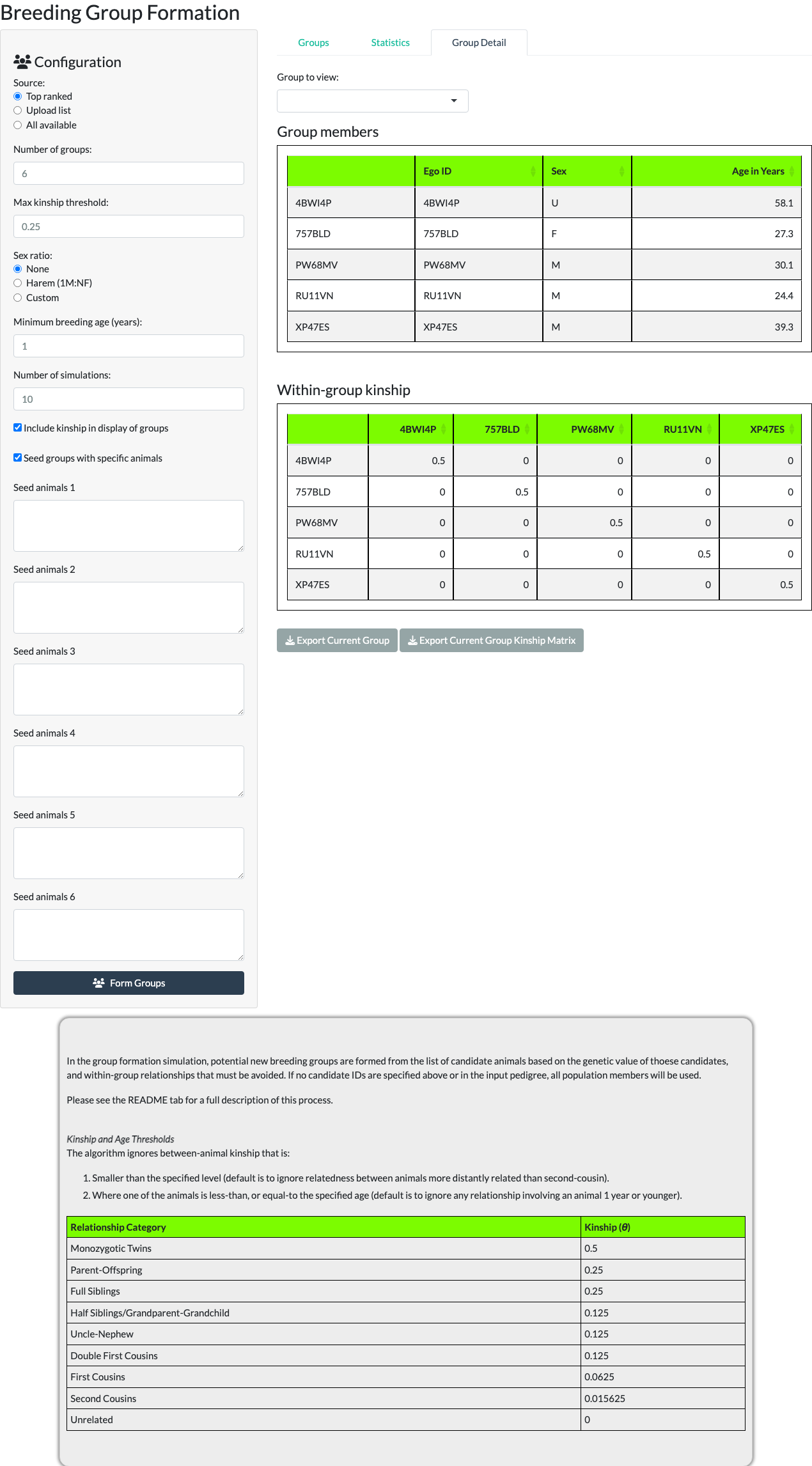
A Statistics sub-tab summarizes all formed groups at once. Groups and their kinship matrices can each be exported individually to a file and location you choose.
If you read a different pedigree, or trim the pedigree on the Pedigree Browser, after groups are formed, a formed group may hold an animal the loaded pedigree no longer has. The Groups, Statistics and Group Detail sub-tabs then show one sentence in place of their tables: “Some animals in these breeding groups are not in the pedigree now loaded (a new file or a trimmed view). Form the groups again, or bring back the earlier pedigree, to see them.”
Ancestry guardrails (issue #168). Centers that manage geographic ancestry – for example keeping Indian-origin and Chinese-origin rhesus lines separate – can upload an ancestry rules file in the Ancestry Guardrails section of the configuration panel (check the box to expand it; the status line beneath always shows what is loaded). Each line of the rules file names two ancestry classifications and a severity: block rules keep matching pairs out of the same group during formation, while flag rules let the groups form and report the matching pairs afterward. After forming groups, the Ancestry sub-tab lists every within-group pairing a rule matched, alongside a coverage summary showing how many grouped animals carry each ancestry classification and which classifications no rule reaches – an animal whose ancestry no rule names participates in no conflict, so the coverage view is how a rule set that quietly covers too little stays visible.
When professional judgment says a block rule should not apply to a particular run – an approved founder import, for example – select the rule and choose Override rule…: a confirmation step requiring a written reason relaxes that one rule for your session (until you clear the override or load a new rules file), and its matched pairings stay in the violations list marked “overridden” rather than disappearing. A Download Audit Manifest button exports the run’s audit record: the rules in effect, any overrides with their reasons, pair counts, and the confirmation warning text verbatim, so the decision trail leaves the tool with the groups.
One practical note on writing rules: pedigree files record “unknown” ancestry in two ways that the standardized vocabulary keeps separate – a truly blank entry becomes UNKNOWN, while unrecognized text (including the literal word “unknown” after re-standardization) becomes OTHER. A center writing a conservative rule for animals without usable ancestry information should therefore name both UNKNOWN and OTHER; the validator warns when a rules file names one without the other, and the example rules file shipped with the package (example_ancestry_rules.csv) models naming both.
Mate Pair Analysis
The Mate Pair Analysis tab (issue #151) is new since the original tutorial-era documentation. It answers a different question than the Breeding Groups tab: not “what multi-animal groups should be formed,” but “for a given, deliberately scoped population, which individual male/female pairs are even eligible to consider, and what do we know about each pair” – a curator-facing worksheet, kept structurally and file-wise separate from group formation.
Choosing a candidate population. Unlike group formation, this tab requires an explicit population scope before it will compute anything – All alive (every animal with no recorded exit date), Top ranked by genetic value (the highest-ranked animals from a completed Genetic Value Analysis run), or a Custom list of pasted IDs. This is a deliberate, evidence-based design choice, not an arbitrary restriction: minimum age alone does not bound the candidate table on real colony data, because a missing recorded age passes the age screen rather than being excluded by it, and a large fraction of animals in a typical studbook have no recorded age at all. Scoping the population first keeps the resulting table both meaningful and responsive.
Set the Minimum breeding age floor and, optionally, check Exclude specific animals to open a text area for animals that should never appear in a pair regardless of any other eligibility screen. Click Find Eligible Pairs to compute the result.
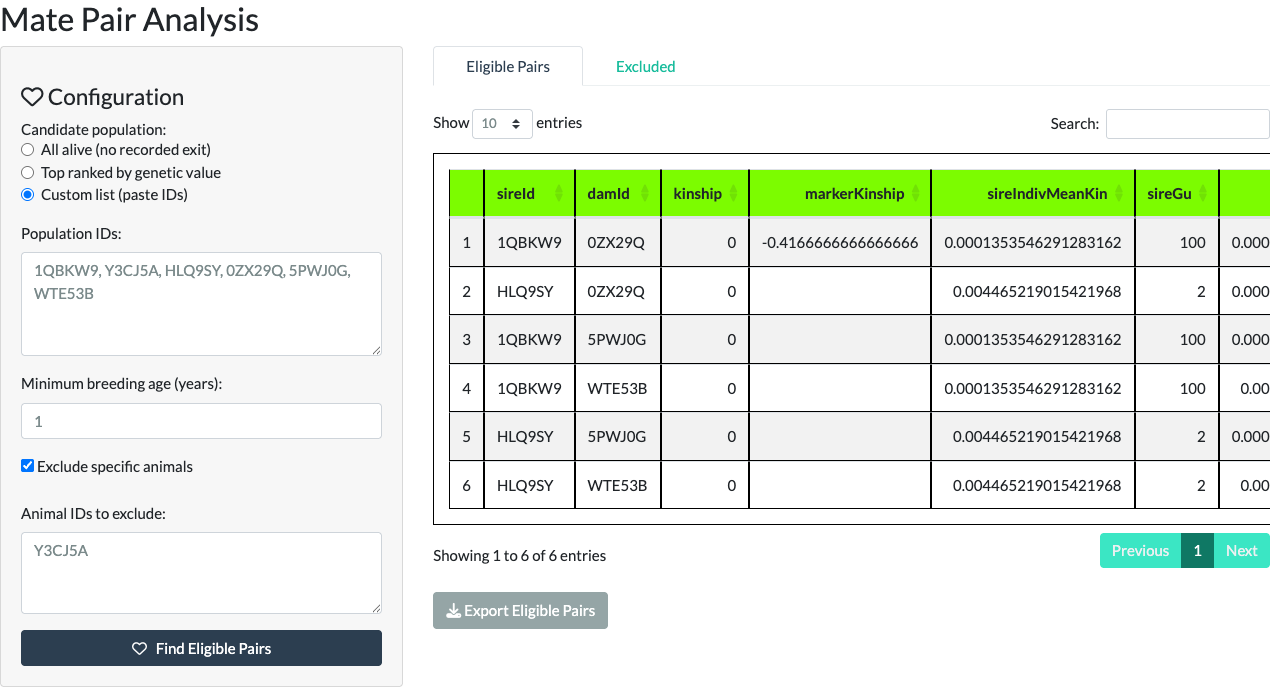
The Eligible Pairs table reports, for every opposite-sex pair surviving the population, age, and exclude-list screens: pedigree kinship, and – when a genotype file has already been uploaded on the Marker Genetics tab – marker-based kinship for that same pair, alongside each parent’s pedigree-based mean kinship and genome uniqueness (the same indivMeanKin/gu values shown on the Genetic Value Analysis tab). No single blended “compatibility score” is computed; sort or filter the raw columns directly, the same way every other ranked table in this application works. The table is sortable and filterable server-side, and its CSV export downloads exactly the rows currently visible after any filter – not the full, unfiltered table.
A separate Excluded tab shows every pair the age or exclude-list screen dropped, together with its reason, so a curator can see why a pair is missing instead of it silently disappearing. Export Excluded Pairs under the table saves them as a CSV file; as with the Eligible Pairs export, the file holds exactly the rows left after any filter.
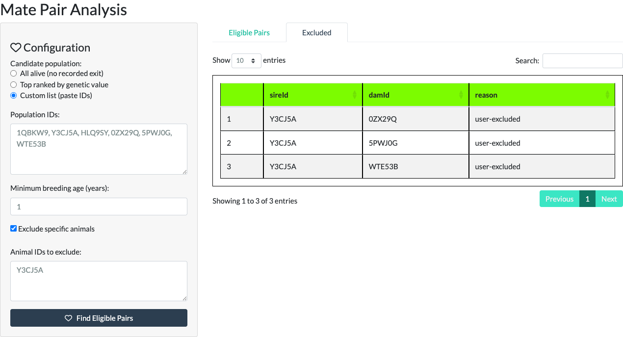
A demographically-eligible pair with very high kinship (e.g. full siblings) is not specially flagged or hidden by this tab – it appears in the Eligible Pairs table exactly like any other pair, with a high kinship value. That value is the signal a curator uses to avoid such a pairing; this tab surfaces the information rather than making the decision for them.
Ancestry guardrails on this tab (issue #169). The ancestry rules you load in the Ancestry Guardrails section of the Breeding Groups tab (described above) also apply here, so a pairing your center keeps apart when forming groups is kept out of the pair list too. There is nothing to upload on this tab. Check Ancestry Guardrails in the configuration panel to expand its section; the status line beneath it always says whether rules are loaded and, if so, how many block and flag rules there are and how many animals carry an ancestry no rule mentions. If the pedigree has no ancestry column the rules cannot apply, and the status line says the guardrails are inactive – the tab then works exactly as it always has. The rules are read when you click Find Eligible Pairs, so loading or changing rules afterward does not rewrite results already on screen; click the button again to apply them.
A pair that matches a block rule moves to the Excluded tab with the reason “ancestry rule”. A pair that matches a flag rule stays in Eligible Pairs, with the matching rule shown beside it (the same columns are in the CSV export). If no eligible pairs remain, the message on screen also says how many pairs the ancestry rules excluded.
When professional judgment says a block rule should not apply to a particular run – an approved founder import, for example – select the rule in the expanded section and choose Override rule…. A confirmation step shows a warning that overriding lets this tab list pairs the rule would otherwise exclude, and requires a written reason; an empty reason is refused. The override lasts for your session on this tab (Breeding Groups keeps its own overrides) until you choose Clear overrides or load a different rules file, and it takes effect the next time you click Find Eligible Pairs. The pairs that rule matches then appear in Eligible Pairs marked “overridden” rather than disappearing.
The Ancestry tab shows, for the run on screen, how many candidate animals carry each ancestry classification and which classifications no rule covers – so a rule set that quietly covers too little stays visible – together with a Download Audit Manifest button. The manifest has one row per rule: the rule, whether it was overridden and the reason given, how many pairs it matched, the animal counts by ancestry classification, and the confirmation warning text verbatim. It always describes the run currently displayed, never a later override, and it is unavailable for a run made with no rules in effect.
Genetic Diversity
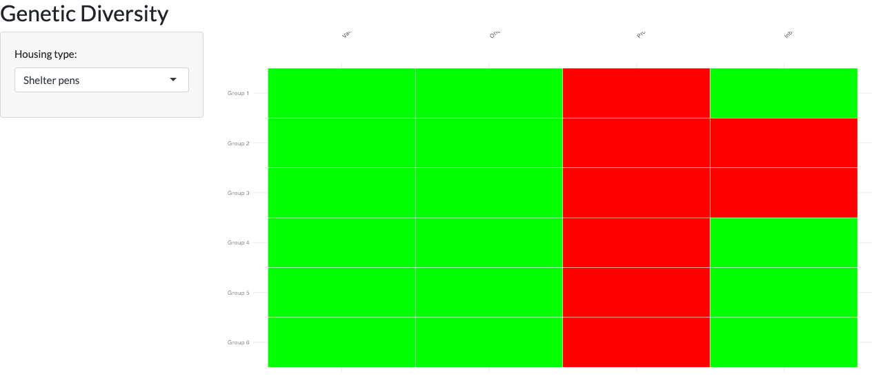
The Genetic Diversity tab (issue #112) is new since the package’s original tutorial-era documentation. It monitors the diversity of breeding groups after they are formed: once groups exist (Breeding Groups tab) and a Genetic Value Analysis has been run, it renders a red/yellow/green heat map with one row per group and one column per metric – Value (the proportion of low-value animals in the group), Origin (Indian- vs. Chinese-origin status, shown only when the pedigree has an ancestry column), Production (births per breeding-age female over the last two calendar years, scored red/yellow/green against cut-offs that depend on the selected Housing type, “Shelter pens” or “Corral”), and Inbreeding (within-group kinship risk involving the group’s male). When some animals fit no group, the last row is that box of animals, named Unused animals as on the Breeding Groups tab, and it is scored like a group. A group with no assessed value, or an undefined Inbreeding result, is scored red rather than shown as healthy, so missing data surfaces instead of hiding as a false green. A breeding-age female is one at least 3 years old. A female with no birth date has no age, so, in both the Production and the Inbreeding column, she counts as a breeding-age female only when the pedigree lists an offspring for her, wherever that offspring is; with no offspring she is left out. A male with no birth date is never counted as a potential mate in the Inbreeding column. A group with no breeding-age females has no Production value, and its cell is gray. When any animal in the groups has no birth date, a note under the heat map says how many, and how many of those females were counted or left out. Until groups are formed and an analysis has run, the tab shows guidance instead of an empty plot. The tab shows a sentence in place of the heat map in one more case: a formed group holds an animal the loaded pedigree no longer has (after reading a different pedigree or trimming the view). Form the groups again to see the heat map.
Marker Genetics
The Marker Genetics tab (issue #130) is new since the original tutorial-era documentation. Every other analysis in nprcgenekeepr estimates kinship from the recorded pedigree; this tab estimates kinship directly from a marker genotype panel instead – an independent check on relatedness that does not depend on the pedigree being complete or correct, matching how NPRC genetics working groups already use SNP panels (e.g. Ancestry-Informative-Marker and Genetic-Management panels) for parentage, kinship, and colony genetic-management decisions in practice.
Upload a marker genotype file with one row per animal x locus (columns id, locus, allele1, allele2 – see the file format guidance on the tab itself) to compute the KING-robust kinship estimator (Manichaikul et al. 2010), which requires biallelic markers and is robust to population substructure. The tab displays a per-animal comparison table: the pedigree-based mean kinship already shown on the Genetic Value Analysis tab, alongside the new marker-based mean kinship – letting a colony manager see at a glance where the two estimates agree or diverge for a given animal.
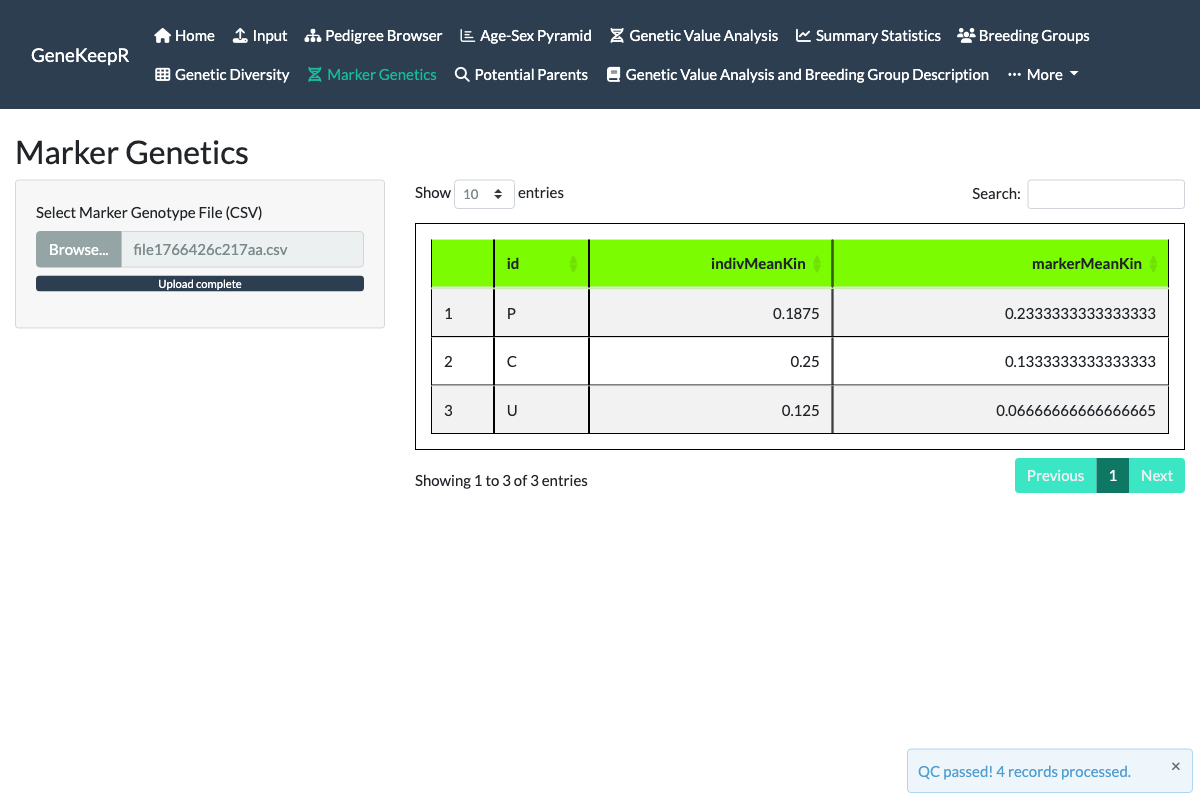
A second Heterozygosity tab (also part of issue #130) surfaces a related but distinct diagnostic from the same uploaded genotype file: each animal’s observed heterozygosity (ho, the fraction of its genotyped loci at which it carries two different alleles) alongside the population’s expected heterozygosity (he, Nei’s gene diversity computed from marker allele frequencies and averaged across loci). Observed running below expected across the population points toward inbreeding or population substructure; observed running above expected points the other way, toward outbreeding.
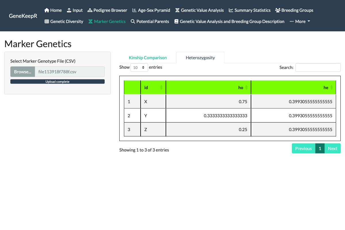
A third Parentage Exclusion tab (also part of issue #130) cross-references the current pedigree’s recorded dam and sire against the same uploaded genotype file: for each animal with a genotyped recorded parent, it counts the marker loci at which the two are Mendelian-inconsistent (both homozygous for a different allele – no shared allele is possible) and flags any recorded parent whose genotype evidence contradicts the pedigree, directly targeting real-world dam/sire misidentification. A single mismatching locus does not trigger a flag on its own, since ordinary genotyping error or mutation can produce an isolated mismatch even for a true parent-offspring pair – the tab flags a recorded parent only once its exclusion count exceeds a conservative, tunable tolerance (3 or more inconsistent loci by default).
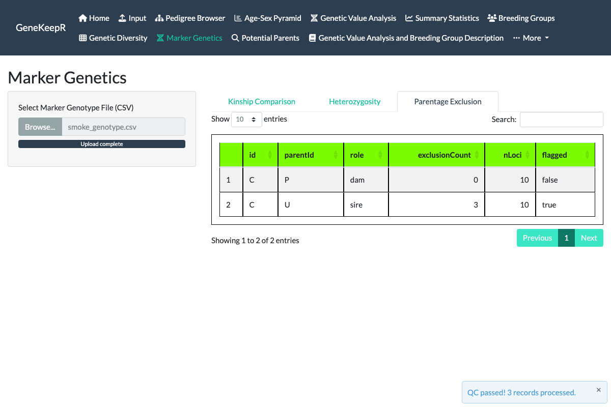
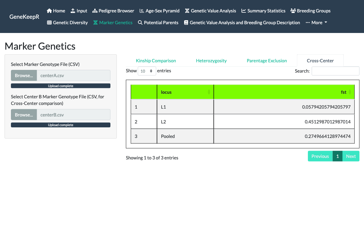
A fourth Cross-Center tab (also part of issue #130) answers a different question than the other three: not “how related are these animals,” but “how genetically differentiated are two separate colonies.” Upload a second marker genotype file for a second center (the first uploaded file becomes “Center A”), and the tab computes Hudson’s Fst – a standard allele-frequency differentiation statistic – at every marker locus genotyped in both centers, plus a single pooled summary value. A value near zero means the two centers’ allele frequencies at that locus are essentially indistinguishable; a larger value (Fst can range up to 1, and can occasionally come out slightly negative due to sampling noise) means the two populations have drifted apart at that marker.
Hudson’s estimator was chosen over the more commonly-cited Weir & Cockerham (1984) estimator specifically because it is not biased by an imbalance between the two centers’ sample sizes – a real concern here, since different centers plausibly submit marker panels for different numbers of animals. The per-locus values are pooled into the single summary as a ratio of sums rather than a simple average, because averaging per-locus ratios directly is a well-documented source of bias for this kind of statistic.
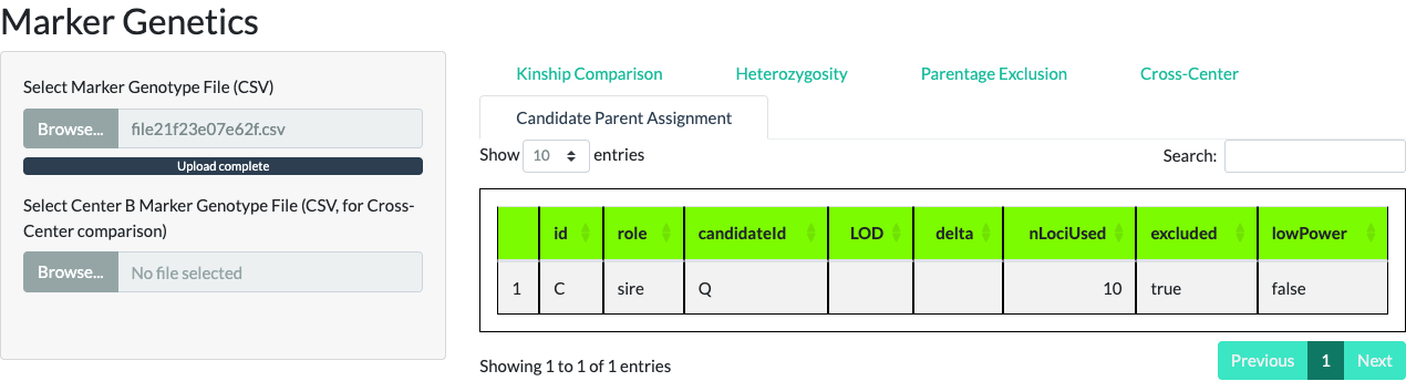
A fifth Candidate Parent Assignment tab (issue #147) picks up directly where the Parentage Exclusion tab leaves off: for every recorded dam or sire that tab flags as Mendelian-inconsistent, this tab ranks candidate replacement parents using a CERVUS-style multilocus likelihood-ratio (LOD) score – the same field-standard method already cited by the Parentage Exclusion tab’s own diagnostic. No new file upload is needed; the tab reads the same genotype file and pedigree already loaded for the rest of the module.
For each flagged animal, every demographically-eligible candidate parent is scored and ranked by LOD (higher is more consistent with the observed genotypes), alongside delta (the gap down to the next-best candidate), nLociUsed (how many loci the comparison actually rests on), excluded (whether this specific candidate is itself Mendelian-inconsistent), and lowPower (whether too few loci were shared to trust the ranking). The tab deliberately does not report a simulation-calibrated percentage confidence – this package’s realistic marker-panel sizes sit inside the range the underlying literature documents as underpowered for that kind of claim, so an uncalibrated raw score is the honest signal to show a curator. Like the Parentage Exclusion tab, this is a diagnostic only: it never rewrites the pedigree’s recorded dam or sire, and any change to the colony’s records remains a curator decision made outside the tool.
Note
What the candidate list needs. Candidate lists come from the same demographic screening the Potential Parents tab uses (age, sex, presence date, gestation window), which needs the pedigree’s
fromCentercolumn; without that column the table is empty, and the tab says so in a notice above the table, in the same words as the Potential Parents tab. For an animal whose recorded parent is present but wrong – the case this tab exists for – the tab sets that recorded parent aside, screens candidates for the freed slot, and keeps the recorded parent in the list, so it appears with its own score beside the others. A curator can also supply a candidate list explicitly (a script-callable option not exposed in this tab).
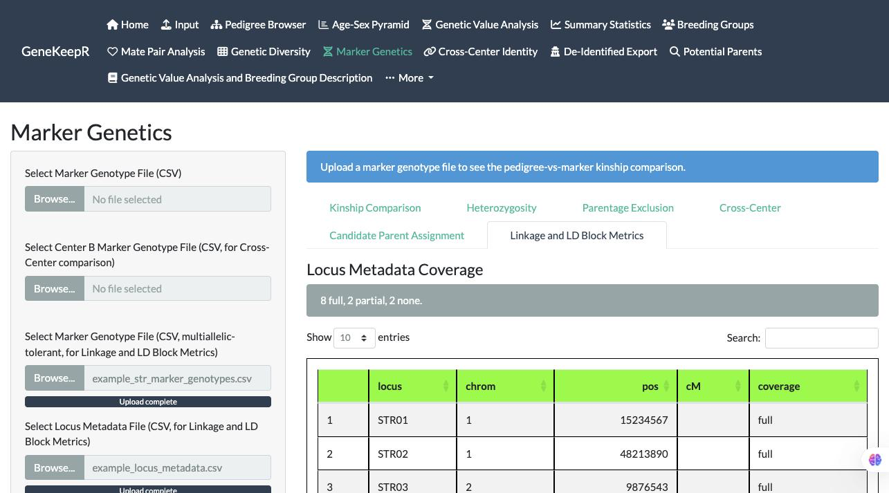
A sixth Linkage and LD Block Metrics tab (issue #153) answers a question the other five tabs deliberately don’t: whether nearby marker loci carry information about relatedness or linkage beyond what each locus contributes independently. It needs its own dedicated marker genotype upload (separate from the file used by the other five tabs, since it tolerates multiallelic panels – e.g. microsatellite/STR panels – that the other tabs’ biallelic-only KING-robust estimator would reject) plus a locus metadata file describing each locus’s chromosome, physical position, and (optionally) genetic-map position.
Uploading the locus metadata file first shows a coverage report: real colony marker panels rarely have complete positional information, so every locus is classified into one of three explicit tiers – full (chromosome and position both known), partial (only one known), or none – rather than silently requiring complete metadata before anything downstream works.
Below the coverage report, two complementary metrics are computed. The Realized Relatedness Variance table is the tab’s primary, genuinely pedigree-valid metric (Hill & Weir 2011): pedigree-based kinship is only an average expected relatedness – the actual proportion of genome shared identical-by-descent between two relatives varies around that average because of Mendelian sampling and linkage, and this table estimates that variance for Parent-Offspring, Full-Sibling, and Half-Sibling pairs given a curator-supplied chromosome count and total genetic-map length (pre-filled with rhesus macaque defaults, adjustable for other species or datasets). It needs no genotype file at all – only the pedigree already loaded elsewhere in the app.
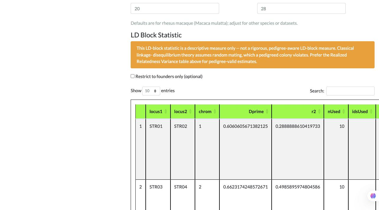
The LD Block Statistic table is a secondary, explicitly-caveated descriptive measure (D’ and r², computed pairwise for same-chromosome loci from the multiallelic genotype upload): classical linkage-disequilibrium theory assumes a randomly-mating population, which a pedigreed colony violates by construction, and no rigorous method that is both pedigree-aware and tolerant of multiallelic data currently exists as a CRAN package. A persistent, non-dismissable banner states this caveat directly above the table – it always accompanies the statistic, since this is a genuine, documented limitation rather than an oversight. An optional checkbox restricts the computation to founder animals only, which reduces (but does not eliminate) the effect of related individuals in the sample.
Because a joint, multi-locus statistic like an LD-block table carries more re-identifying power than a single-locus summary (not less), any exported LD-block table is de-identified and routed through the same curator confirm-gate pattern as the De-Identified Export tab below: generate a preview, confirm via a modal dialog, then download. The Realized Relatedness Variance table has no export control – like the other five Marker Genetics tabs, it is a report-only, on-screen diagnostic.
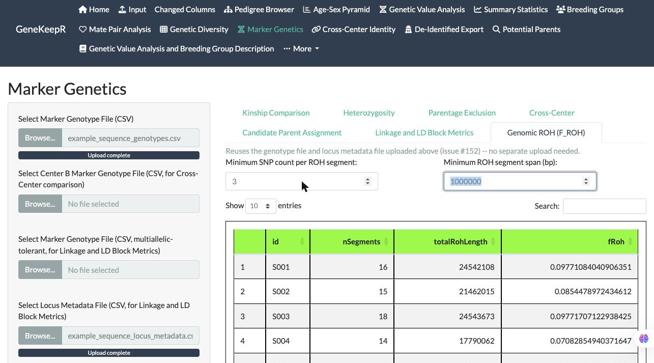
A seventh Genomic ROH (F_ROH) tab (issue #152, the final slice, closing that issue) computes a marker-based inbreeding estimate independent of the recorded pedigree: the genomic inbreeding coefficient F_ROH, derived from Runs of Homozygosity (ROH) – long stretches of consecutive homozygous loci that are unlikely to occur by chance and typically indicate the two chromosome copies at that stretch are identical by descent. Unlike the Linkage and LD Block Metrics tab above, this one needs no separate upload: it reuses the same genotype file already uploaded for the Kinship Comparison tab (now validated by a rule set sized for larger, sequence-scale panels) and the same locus metadata file already uploaded for the Linkage and LD Block Metrics tab, since both tabs share the same locus/chrom/pos vocabulary by design.
A run of consecutive homozygous, non-missing loci (ordered by physical position along each chromosome) qualifies as an ROH segment only if it meets both a minimum SNP-count threshold and a minimum base-pair span threshold – the same field-standard dual-threshold convention PLINK uses, adjustable via the two fields above the table (pre-filled with 50 SNPs, a scaled-down version of PLINK’s default of 100, and 1,000,000 base pairs, which is PLINK’s own default). F_ROH is the proportion of the genome covered by qualifying segments.
F_ROH is calculated only from the loci that are in the genotype file. If the locus metadata file lists loci with a chromosome and position that are not in the genotype file, a notice above the table says how many and names them, because every animal’s F_ROH is then relative to a shorter stretch of genome than the locus file describes.
Like the Linkage and LD Block Metrics tab, any export from this tab is de-identified and routed through the same curator confirm-gate pattern: generate a preview, confirm via a modal dialog, then download. Three artifacts are available – the de-identified genotype matrix, the de-identified F_ROH table, and a transformation manifest recording the export’s own timestamp, package version, and the SNP-count/base-pair thresholds used, mirroring the De-Identified Export tab’s own manifest convention below.
An eighth MHC Haplotype Reporting tab (issue #148) reports how common each MHC haplotype is in the colony, which haplotypes are rare, and which animals carry the rare ones – so a manager can see which animals matter before a rare haplotype is lost. It has its own upload, separate from the marker genotype files above: a CSV with one row per animal, an id column first, then that animal’s two haplotype designations (the bundled obfuscated_rhesus_mhc_breeder_genotypes.csv example is exactly this shape). Designations are used exactly as written; a trailing ? marks a provisional call, which is counted and shown but left out of the frequencies. A persistent banner states that this is descriptive reporting of the designations you supply, not a replacement for the pedigree-based statistics elsewhere in the app.
A haplotype is flagged rare when its frequency is at or below the first threshold (default 0.01) or it is carried by no more than the second (default 2 animals). Both thresholds sit next to the tables and can be changed. The carrier rule matters most in small colonies: with 31 animals no haplotype can reach a frequency as low as 0.01, so on the bundled example it is the carrier rule that flags 26 of the 33 haplotypes. A line above the tables gives the counts behind the frequencies (animals, missing and provisional designations, and the number of certain designations used), and, once a pedigree is loaded, how many pedigree animals have a designation.
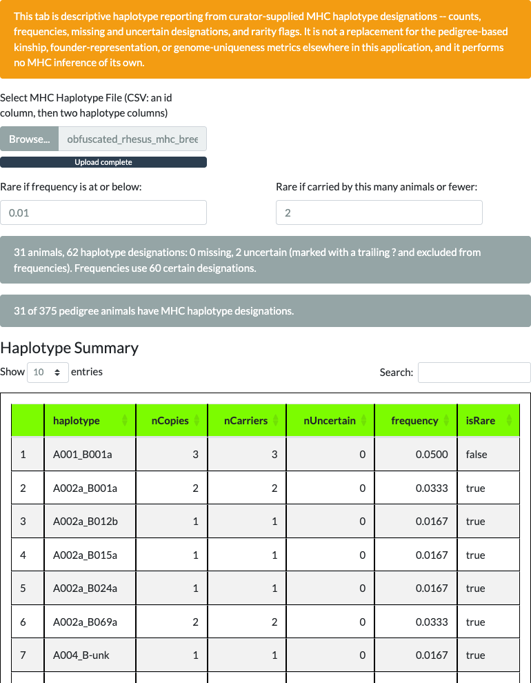
Exports from this tab go through the same curator confirm-gate as the tabs above: generate a preview, confirm in the dialog, then download the haplotype summary, the rare-haplotype carrier list with animal ids replaced by the pedigree’s de-identification aliases, and a manifest recording the thresholds and counts in force. The summary is gated too, because a paired MHC type can identify an animal on its own. Every animal in the MHC file must be in the loaded pedigree before exporting; if any is missing, the tab says so and does not build the export.
Cross-Center Identity
The Cross-Center Identity tab (issue #149) addresses a different problem than any other tab: a colony animal transferred between centers is often recorded twice, once under each center’s own id namespace, so the transferred animal shows up at the receiving center as an artificial founder – its real parents, known at the origin center, are lost from every downstream analysis. This tab operationalizes a reviewed fix: a curator uploads both centers’ pedigrees plus their own explicit id-mapping table (which id at Center A is the same physical animal as which id at Center B), and the tool safely merges the two records, restoring the real lineage. Like every other identity-sensitive feature in nprcgenekeepr, this tool never guesses identity from matching id strings or genetic data – only the mapping a curator explicitly supplies is ever merged.
The workflow has three steps, each its own tab:
-
Validation. Upload Center A’s pedigree, Center B’s pedigree, and the mapping file (columns
idA/idB), then click Validate Mapping. Every problem is surfaced at once – not just the first one found – so a mapping file with several unrelated mistakes (a duplicate mapping row, an id that doesn’t exist in either pedigree, an id present at both centers but never declared in the mapping, a Center B animal whose id the mapping already gives to a different Center A animal, or two centers recording different parents for the same mapped animal) can be fixed in one pass instead of being rejected and resubmitted repeatedly. - Preview. Once the mapping validates clean, this tab computes the actual proposed merge and shows a lineage-change table: for each mapped pair, both centers’ originally-recorded sire/dam alongside the resolved sire/dam and which center’s record it came from. Clicking Confirm Merge opens a confirmation dialog summarizing the mapped-pair and final-merged-row counts before anything is unlocked for export.
- Export. Once confirmed, five artifacts become downloadable: the Merged Pedigree itself, an echo of the confirmed Mapping, the Validation Results (useful as an audit artifact even when clean – proof no problems were found), the Merge Summary (the same lineage-change table from the Preview tab), and a Provenance record (timestamp, the three uploaded file names, package version, and per-merged-animal source counts).
This is a standalone review/export tool: the merged pedigree is a downloadable CSV, not automatically fed into the rest of the application. A curator who wants the merged result to drive genetic value, breeding-group, or diversity analysis re-uploads the exported “Merged Pedigree” file through the Input tab’s existing pedigree-file path.
De-Identified Export
The De-Identified Export tab (issue #150) supports approved external data sharing: producing a relationship-preserving, de-identified copy of the pedigree already loaded in the current session, without a separate upload. It reuses the package’s existing, already-tested de-identification primitives (obfuscateId(), obfuscateDate(), obfuscatePed()) rather than any new anonymization logic.
The workflow has two steps:
- Configure & Preview. Set the alias-id length, the maximum date shift (in days), and whether each individual’s dates should shift together (linked, the recommended default) or independently. Linked shifting preserves an individual’s exact inter-date gaps (e.g. birth-to-exit) – independent shifting can, on a short-lived individual, invert that order and produce a negative recomputed age; this is why linked shifting is the default, not merely an option. Clicking Generate Preview shows the full de-identified output before anything is exported, so a curator sees exactly what would leave the building. Displayed ages are recomputed from the shifted dates, not the original recorded values.
- Export. Clicking Confirm Export opens a dialog carrying an explicit institutional-responsibility disclaimer – this app’s first – making clear that de-identification is not authorization: confirming your institution’s data-sharing policies permit the export and its intended recipient(s) remains the curator’s own responsibility, not the tool’s. Once confirmed, three artifacts become downloadable: the de-identified pedigree itself, a transformation manifest (the parameters used, row count, and timestamp – never the id map or any raw pre-obfuscation value, so it is safe to attach as evidence of how an export was produced without revealing what it replaced), and a distinctly labeled re-identification key (“DO NOT SHARE”) mapping each alias back to its original id. The key downloads as its own, separately labeled file so it is never mistaken for a shareable artifact.
Fields outside id, dam, sire, dates, and name (e.g. origin, status) pass through unchanged – disclosed in both the warning text and the manifest, not silently scrubbed, since scrubbing them was never part of this tool’s scope. As with Cross-Center Identity above, “curator-controlled” here means a confirmation dialog and warning text, not real access control: this package has no user-identity or role infrastructure to enforce authorization against, and inventing one was explicitly out of scope for this feature.
Potential Parents
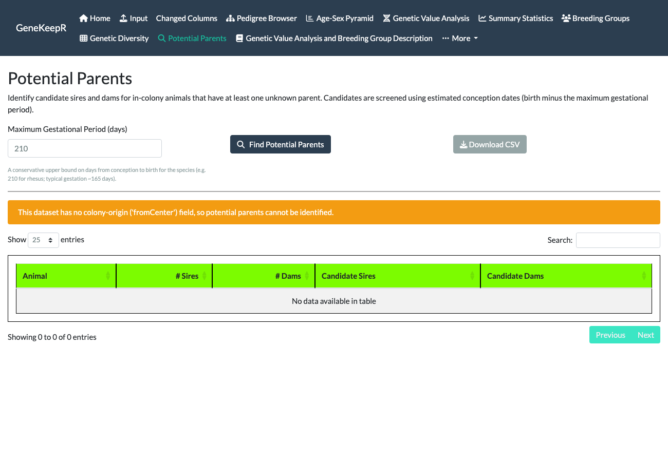
The Potential Parents tab (issue #48) is also new since the original tutorial-era documentation. It proposes candidate sires and dams for in-colony animals recorded with at least one unknown parent, screening candidates by estimated conception date (birth date minus a Maximum Gestational Period in days – prefilled from the pedigree’s recorded species, e.g. 210 days for rhesus, and adjustable) and by the same minimum sire/dam breeding ages set on the Input tab. Results are shown in a sortable table and downloadable as CSV.
Note
Fixed before publication. An earlier draft of this walkthrough found the shipped
data(examplePedigree)had nofromCenter(colony-origin) column, which this feature requires to identify which animals are in-colony candidates versus animals whose origin is unrecorded – so this section could only show the application’s own correctly-degraded empty-result response rather than a populated example. Fixed by deriving a realfromCentercolumn for the shipped example pedigree from its existingorigin/recordStatusfields; the screenshot below now shows real results. If your own pedigree is missing this column, you will see that same correctly-degraded response instead of the populated table below.
Selecting Find Potential Parents against the full example pedigree reports “Found candidate parents for 1,587 animal(s) with at least one unknown parent,” in a sortable, paginated, CSV-downloadable table.
Genetic-Health Trends
The Genetic-Health Trends tab (issue #167) turns the one-time snapshots on the Genetic Value Analysis tab into a longitudinal record: a running history of dated colony snapshots that lets you see whether the colony’s genetic health is improving or eroding over time.
The workflow has three parts:
- Snapshot history. Upload a snapshot-history file (the package ships a worked example file for this tab) or start recording a new one. Each row is one dated snapshot – mean kinship, founder representation, genome uniqueness, and the population’s make-up – for a single membership rule (the whole pedigree, or a smaller population: the living animals, or the focal animals you entered).
- Generate Snapshot. After running Genetic Value Analysis on the Genetic Value Analysis tab, clicking Generate Snapshot here records a new dated row from that analysis and appends it to the history. The membership rule is filled in automatically from the analysis you just ran – it is not a setting you have to get right by hand.
- Trends and comparisons. The Trends tab plots every recorded value over time, with shaded bands showing the uncertainty that comes from repeated random sampling. The Deltas tab lists what changed, value by value, between any two recorded dates you choose. Both flag snapshots recorded under different settings or package versions, so a jump in the numbers is not mistaken for a real change in the colony. The updated history and the delta table are both downloadable for record-keeping.
Note
This section is text-only, matching the established precedent for a straightforward new-tab addition (see the Cross-Center Identity section above); the tab’s behavior is fully covered by the package’s automated tests and a live end-to-end run, not only by this description.
Conclusion
This article covered why nprcgenekeepr exists, how its five function groups map onto the Shiny application’s tabs and onto a scriptable R API, and what it looks like to actually use every tab of that application against the package’s own example data. For more depth on any one capability, see the feature articles in Table 1; for the story of how the current modular application came to be, see “Engineering nprcgenekeepr 2.0.0”. This article’s own preparation surfaced and fixed three production issues along the way – an Excel-upload sire/dam corruption defect, a non-functional “Custom” breeding-group sex ratio, and a shipped example pedigree missing the column the Potential Parents tab needs to demonstrate populated results – each described where it arose in Section 3. Please report any further questions, comments, or bugs through the GitHub issue tracker.
Work on this package up to and including version 1.0 was supported in part by NIH grants P51 RR13986 to the Southwest National Primate Research Center and P51 OD011092 to the Oregon National Primate Research Center.